Week 4: Non-linear regression

PLS 206 — the code behind the lectures

Author

Grey Monroe

One page for the whole week. It follows the slides (Week4_Nonlinear.pptx) in order, and has the code behind every figure and number in the lecture, with the output underneath.

To run it yourself, download either version and open it in RStudio. It reads the data straight from the course website, so there is no file to download and no working directory to set:

Week4_Nonlinear.R: the plain script. Each block is tagged [CORE], [HANDY], or [DEMO] in a comment.
Week4_Nonlinear.qmd: this page as a Quarto notebook (open in RStudio, run chunk by chunk, or click Render).

Every block of code on this page carries one of three labels:

Core The analysis. Code you would run on your own data: fit the model, read the output, check the diagnostics, report it. Start here for the problem sets.
Handy Useful, not essential. Wrangling, plotting, and small helpers that make the core easier. Worth knowing; skip on a first read.
Demo For the lecture only. Simulated data, sums done by hand, and the code behind slide figures. It shows why the core works. Folded: click to open.

# install.packages(c("ggplot2", "mgcv", "gratia", "patchwork"))
library(ggplot2)
library(mgcv)

Which tool for which question

You want…	Use
An optimum, or a test for a bend	`lm(y ~ x + I(x^2))`
How many polynomial degrees you need	`lm(y ~ poly(x, d))`
A curve inside `lm` / `glm` / `lmer`, with fixed df	`ns(x, df)` in the formula
The shape, with the wiggliness chosen by the data	`gam(y ~ s(x), method = "REML")`
A parameter with biological meaning	`nls()`

Part A. Bend the line

1) The data: seedlings in growth chambers

300 wheat seedlings, one pot each, grown for 14 days at a constant temperature between 8 and 42 °C. Two varieties: standard and a heat-tolerant line. Measured: shoot dry mass (mass_mg, mg) and whether the leaves showed damage (damaged: 1 = yes, 0 = no). Simulated. Parts A to D use the standard variety only (150 pots).

seedlings <- read.csv("https://greymonroe.github.io/PLS_206/data/seedling_temp.csv")
std <- subset(seedlings, variety == "standard")
head(std)

  pot  variety temp mass_mg damaged
1   1 standard 12.9    35.0       1
2   2 standard 28.2    52.8       1
4   4 standard 15.1    46.5       0
5   5 standard 14.0    35.9       0
6   6 standard 28.5    60.7       0
9   9 standard 10.6    29.2       0

nrow(std)

[1] 150

ggplot(std, aes(temp, mass_mg)) +
  geom_point(colour = "grey40") +
  labs(x = "Temperature (°C)", y = "Shoot dry mass (mg)") +
  theme_classic()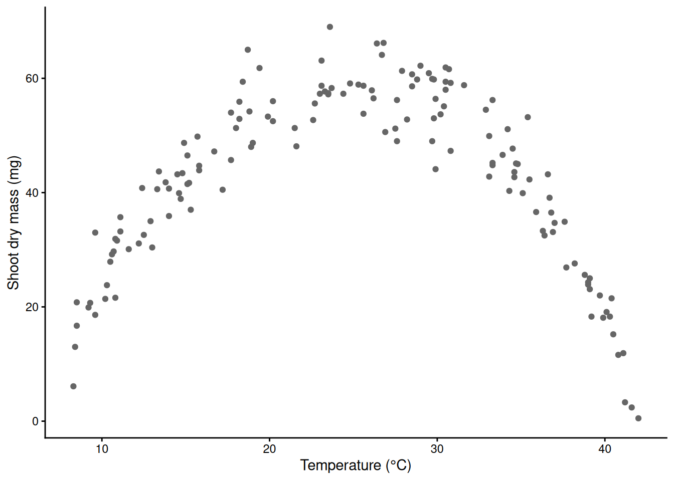

2) A straight line, and its residuals

m_lin <- lm(mass_mg ~ temp, data = std)
summary(m_lin)   # slope p = 0.59, R-squared 0.002: the line sees nothing


Call:
lm(formula = mass_mg ~ temp, data = std)

Residuals:
    Min      1Q  Median      3Q     Max 
-41.038 -10.882   2.596  12.935  26.218 

Coefficients:
            Estimate Std. Error t value Pr(>|t|)    
(Intercept) 44.37849    3.42270  12.966   <2e-16 ***
temp        -0.06764    0.12660  -0.534    0.594    
---
Signif. codes:  0 '***' 0.001 '**' 0.01 '*' 0.05 '.' 0.1 ' ' 1

Residual standard error: 15.54 on 148 degrees of freedom
Multiple R-squared:  0.001925,  Adjusted R-squared:  -0.004819 
F-statistic: 0.2855 on 1 and 148 DF,  p-value: 0.5939

A big p-value is not “no relationship”. It is no evidence for a straight-line relationship. Always look at the residuals.

std$resid_lin <- resid(m_lin)
ggplot(std, aes(temp, resid_lin)) +
  geom_point(colour = "grey40") +
  geom_hline(yintercept = 0, linetype = 2) +
  geom_smooth(method = "loess", se = FALSE, colour = "red") +   # a guide for the eye
  labs(x = "Temperature (°C)", y = "Residual (mg)") +
  theme_classic()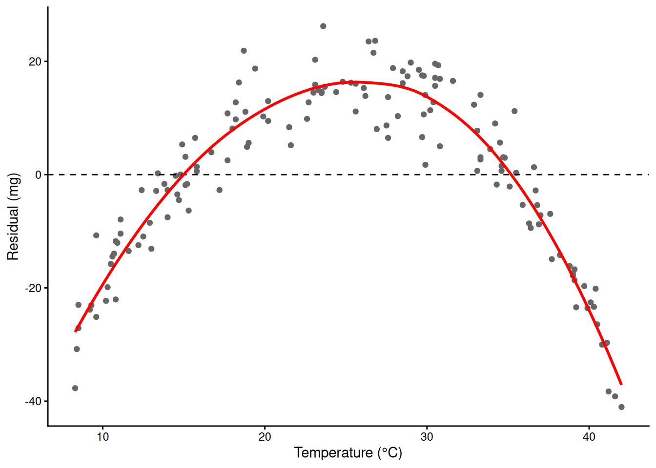

A frown: the line overpredicts at both ends and underpredicts in the middle. The shape is wrong.

3) A helper for every plot: fitted values with a 95% CI

Every model this week gets the same picture: the raw data, the fitted curve, and its 95% confidence band. predict(se.fit = TRUE) gives a fitted value and a standard error on the link scale; the band is fit ± 1.96 SE (or a t quantile for lm()), and the family’s inverse link puts it back on the scale of y. One helper does it for lm(), glm() and gam().

fit_ci <- function(model, newdata, level = 0.95) {
  p <- predict(model, newdata = newdata, se.fit = TRUE)   # link scale for glm and gam
  q <- if (inherits(model, "glm")) qnorm(1 - (1 - level) / 2) else qt(1 - (1 - level) / 2, df.residual(model))
  inv <- family(model)$linkinv                            # identity for lm and Gaussian models
  fit <- as.numeric(p$fit); se <- as.numeric(p$se.fit)
  data.frame(newdata, fit = inv(fit), lwr = inv(fit - q * se), upr = inv(fit + q * se))
}
grid <- data.frame(temp = seq(min(std$temp), max(std$temp), by = 0.05))   # temperatures to predict at (the data range)

ggplot(std, aes(temp, mass_mg)) +
  geom_point(colour = "grey50") +
  geom_ribbon(data = fit_ci(m_lin, grid), aes(temp, ymin = lwr, ymax = upr),
              inherit.aes = FALSE, fill = "blue", alpha = 0.2) +
  geom_line(data = fit_ci(m_lin, grid), aes(temp, fit), colour = "blue", linewidth = 1) +
  labs(x = "Temperature (°C)", y = "Shoot dry mass (mg)") +
  theme_classic()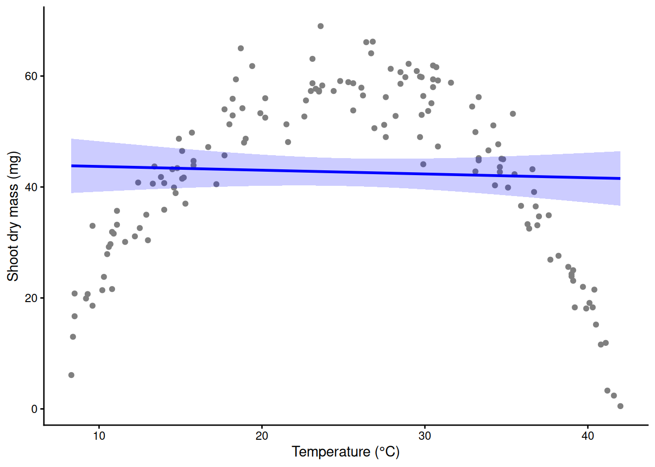

(A gam() object inherits from glm, so it gets the normal quantile too.)

4) Logs and links are already curves

Last week’s logistic and Poisson regressions are straight lines on the link scale, which become curves on the scale of the data. Here are the Week 3 rust and aphid models again.

Demo: last week’s GLMs drawn as curves

trial <- read.csv("https://greymonroe.github.io/PLS_206/data/wheat_trial.csv")
m_rust <- glm(rust ~ nitrogen, family = binomial, data = trial)
m_aph  <- glm(aphids ~ nitrogen, family = poisson, data = trial)
g_n <- data.frame(nitrogen = 0:200)
p1 <- ggplot(trial, aes(nitrogen, rust)) +
  geom_jitter(width = 0, height = 0.03, colour = "grey50") +
  geom_ribbon(data = fit_ci(m_rust, g_n), aes(nitrogen, ymin = lwr, ymax = upr), inherit.aes = FALSE,
              fill = "red", alpha = 0.2) +
  geom_line(data = fit_ci(m_rust, g_n), aes(nitrogen, fit), colour = "red", linewidth = 1) +
  labs(x = "Nitrogen (kg N/ha)", y = "P(rust)", title = "Logistic: S-curve") +
  theme_classic()
p2 <- ggplot(trial, aes(nitrogen, aphids)) +
  geom_point(colour = "grey50") +
  geom_ribbon(data = fit_ci(m_aph, g_n), aes(nitrogen, ymin = lwr, ymax = upr), inherit.aes = FALSE,
              fill = "purple", alpha = 0.2) +
  geom_line(data = fit_ci(m_aph, g_n), aes(nitrogen, fit), colour = "purple", linewidth = 1) +
  labs(x = "Nitrogen (kg N/ha)", y = "Aphids per 10 tillers", title = "Poisson: exponential") +
  theme_classic()
library(patchwork)
p1 + p2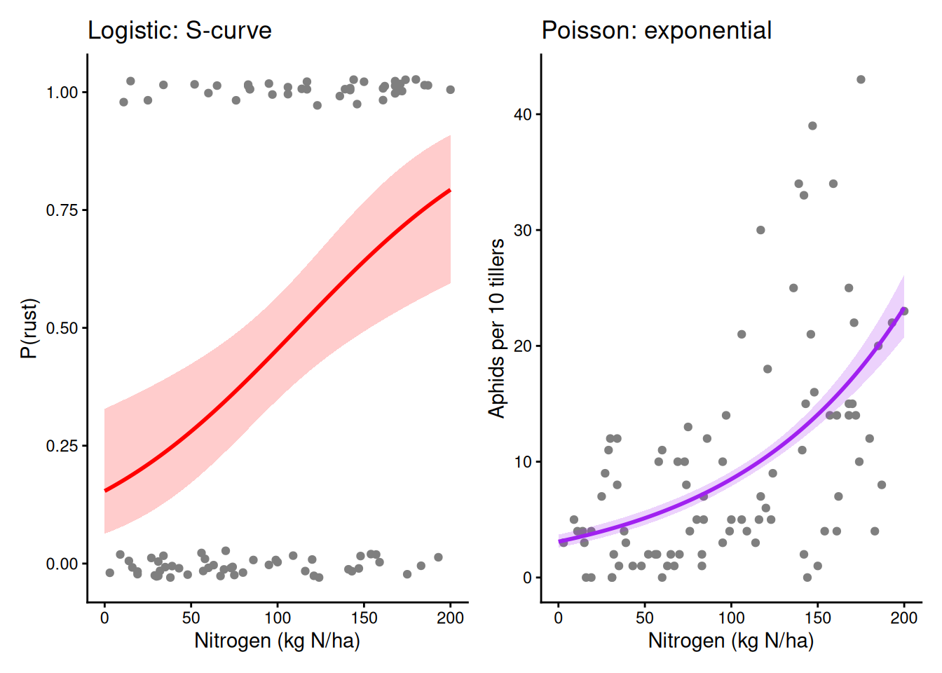

5) The whole trick: a quadratic

Make a new column from x, here temperature squared, and give it a coefficient. I() tells R to do the arithmetic instead of reading ^ as formula syntax. The model is still linear in the coefficients, so lm() fits it.

head(cbind(temp = std$temp, temp2 = std$temp^2))   # the new column

     temp  temp2
[1,] 12.9 166.41
[2,] 28.2 795.24
[3,] 15.1 228.01
[4,] 14.0 196.00
[5,] 28.5 812.25
[6,] 10.6 112.36

m_quad <- lm(mass_mg ~ temp + I(temp^2), data = std)
summary(m_quad)   # temp^2 negative: the curve bends down; R-squared 0.002 -> 0.905


Call:
lm(formula = mass_mg ~ temp + I(temp^2), data = std)

Residuals:
     Min       1Q   Median       3Q      Max 
-11.0866  -2.8436  -0.5789   3.2740  13.1977 

Coefficients:
            Estimate Std. Error t value Pr(>|t|)    
(Intercept) -44.1887     2.5967  -17.02   <2e-16 ***
temp          8.4626     0.2316   36.53   <2e-16 ***
I(temp^2)    -0.1719     0.0046  -37.36   <2e-16 ***
---
Signif. codes:  0 '***' 0.001 '**' 0.01 '*' 0.05 '.' 0.1 ' ' 1

Residual standard error: 4.812 on 147 degrees of freedom
Multiple R-squared:  0.9049,    Adjusted R-squared:  0.9036 
F-statistic: 699.5 on 2 and 147 DF,  p-value: < 2.2e-16

ggplot(std, aes(temp, mass_mg)) +
  geom_point(colour = "grey50") +
  geom_ribbon(data = fit_ci(m_quad, grid), aes(temp, ymin = lwr, ymax = upr),
              inherit.aes = FALSE, fill = "blue", alpha = 0.2) +
  geom_line(data = fit_ci(m_quad, grid), aes(temp, fit), colour = "blue", linewidth = 1) +
  labs(x = "Temperature (°C)", y = "Shoot dry mass (mg)") +
  theme_classic()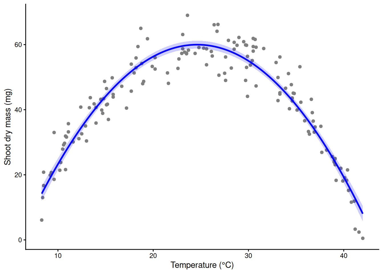

6) The vertex: an estimated optimum

The top of the parabola is where its slope, β1 + 2β2·temp, is zero: temp* = −β1 / (2β2). In a fertilizer trial the same formula gives an optimal nitrogen rate.

b <- coef(m_quad)
vertex <- -b[2] / (2 * b[3])
vertex                                            # about 24.6 °C; the true optimum is 26

    temp 
24.61863

predict(m_quad, data.frame(temp = vertex))        # predicted mass at the top

    temp 
59.98064

std$resid_quad <- resid(m_quad)
ggplot(std, aes(temp, resid_quad)) +
  geom_point(colour = "grey40") +
  geom_hline(yintercept = 0, linetype = 2) +
  geom_smooth(method = "loess", se = FALSE, colour = "red") +
  labs(x = "Temperature (°C)", y = "Residual from the quadratic (mg)") +
  theme_classic()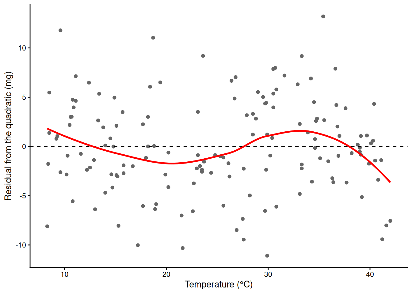

Still a pattern: a parabola is symmetric about its peak, and this curve rises slowly and crashes fast. That is why the vertex sits below the true optimum.

7) Higher polynomials and their edges

More columns: temp³, temp⁴, and so on. poly(temp, d, raw = TRUE) builds them all.

m_p4  <- lm(mass_mg ~ poly(temp, 4, raw = TRUE), data = std)
m_p10 <- lm(mass_mg ~ poly(temp, 10, raw = TRUE), data = std)
sapply(c(1, 2, 3, 4, 6, 10), function(d)
  summary(lm(mass_mg ~ poly(temp, d, raw = TRUE), data = std))$r.squared)   # R-squared by degree

[1] 0.001925166 0.904914918 0.912070574 0.915886927 0.916250731 0.918305050

Beyond the data, a degree-10 polynomial flaps:

Demo: a degree-10 polynomial from 4 to 46 °C

wide <- data.frame(temp = seq(4, 46, by = 0.1))
ci10 <- fit_ci(m_p10, wide)
ggplot(std, aes(temp, mass_mg)) +
  annotate("rect", xmin = min(std$temp), xmax = max(std$temp), ymin = -Inf, ymax = Inf, fill = "grey92") +
  geom_point(colour = "grey50") +
  geom_ribbon(data = ci10, aes(temp, ymin = lwr, ymax = upr), inherit.aes = FALSE, fill = "red", alpha = 0.2) +
  geom_line(data = ci10, aes(temp, fit), colour = "red", linewidth = 1) +
  coord_cartesian(ylim = c(-40, 120)) +
  labs(x = "Temperature (°C)", y = "Shoot dry mass (mg)", title = "Degree 10; shaded = range of the data") +
  theme_classic()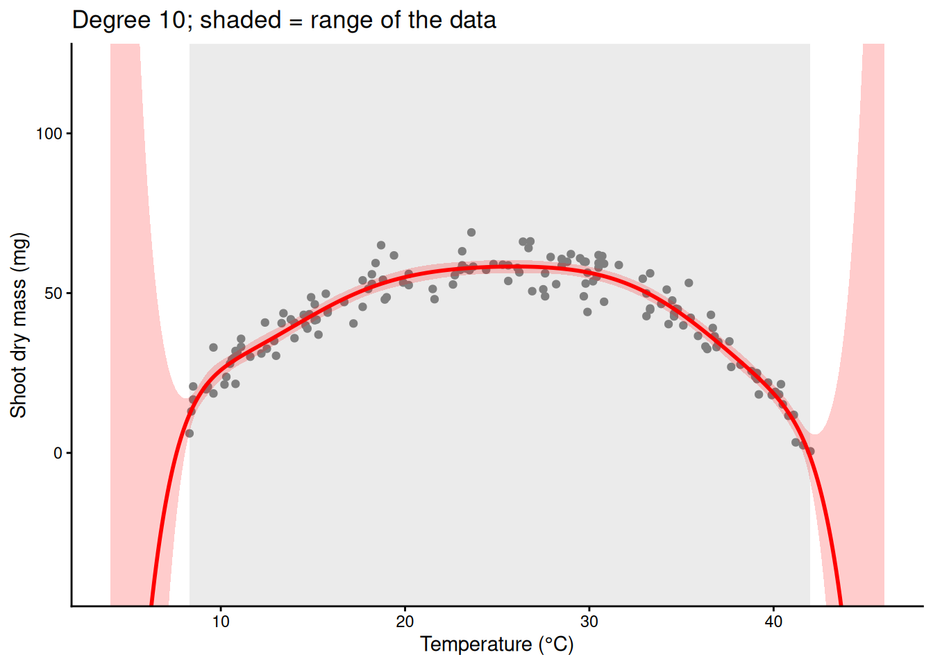

Polynomial columns are global: every power of temperature is non-zero across the whole range, and the big powers are dominated by the hot end. Compare the local spline columns of section 10.

Demo: polynomial columns are global, spline columns are local

library(splines)
tt <- seq(8, 42, by = 0.1)
P <- sapply(1:6, function(d) tt^d / 42^d)   # temp, temp^2, ... scaled to 0-1
B <- bs(tt, df = 6)
cols <- rbind(data.frame(temp = tt, value = as.vector(P), column = factor(rep(1:6, each = length(tt))), type = "Powers: temp, temp^2, ..., temp^6"),
              data.frame(temp = tt, value = as.vector(B), column = factor(rep(1:6, each = length(tt))), type = "Spline: bs(temp, df = 6)"))
ggplot(cols, aes(temp, value, colour = column)) +
  geom_line(linewidth = 1) +
  facet_wrap(~ type) +
  labs(x = "Temperature (°C)", y = "Column value (scaled)") +
  theme_classic() + theme(legend.position = "none")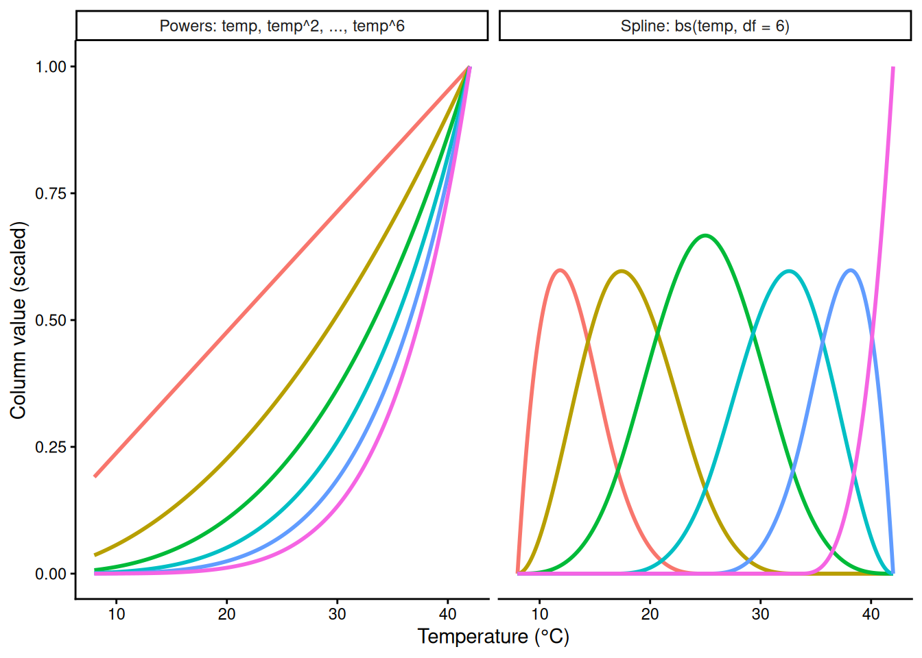

8) Raw vs orthogonal polynomials

Reference. poly(temp, 3) builds orthogonal polynomials: rescaled columns that are uncorrelated with each other. poly(temp, 3, raw = TRUE) builds plain temp, temp², temp³. Same fitted curve, different coefficients. If you will interpret or plug in coefficients (like the vertex), use raw = TRUE.

m_orth <- lm(mass_mg ~ poly(temp, 3), data = std)
m_raw  <- lm(mass_mg ~ poly(temp, 3, raw = TRUE), data = std)
coef(m_orth)

   (Intercept) poly(temp, 3)1 poly(temp, 3)2 poly(temp, 3)3 
     42.680000      -8.301435    -179.787909     -16.004561

coef(m_raw)

               (Intercept) poly(temp, 3, raw = TRUE)1 
             -23.864101723                5.405792771 
poly(temp, 3, raw = TRUE)2 poly(temp, 3, raw = TRUE)3 
              -0.037905217               -0.001777808

all.equal(fitted(m_orth), fitted(m_raw))   # TRUE: the same curve

[1] TRUE

Part B. Splines

9) Pieces joined at knots

Cut the temperature axis at knots and fit something simple in each piece. Each piece listens only to its own data, but separate pieces jump at the knots.

Demo: a separate straight line in each piece

knots <- c(15, 22, 29, 36)
std$piece <- cut(std$temp, c(-Inf, knots, Inf))
m_pieces <- lm(mass_mg ~ piece * temp, data = std)
g_pc <- data.frame(temp = grid$temp, piece = cut(grid$temp, c(-Inf, knots, Inf)))
ci_pc <- fit_ci(m_pieces, g_pc)
ggplot(std, aes(temp, mass_mg)) +
  geom_point(colour = "grey50") +
  geom_vline(xintercept = knots, linetype = 2, colour = "grey60") +
  geom_ribbon(data = ci_pc, aes(temp, ymin = lwr, ymax = upr, group = piece), inherit.aes = FALSE,
              fill = "blue", alpha = 0.2) +
  geom_line(data = ci_pc, aes(temp, fit, group = piece), colour = "blue", linewidth = 1) +
  labs(x = "Temperature (°C)", y = "Shoot dry mass (mg)") +
  theme_classic()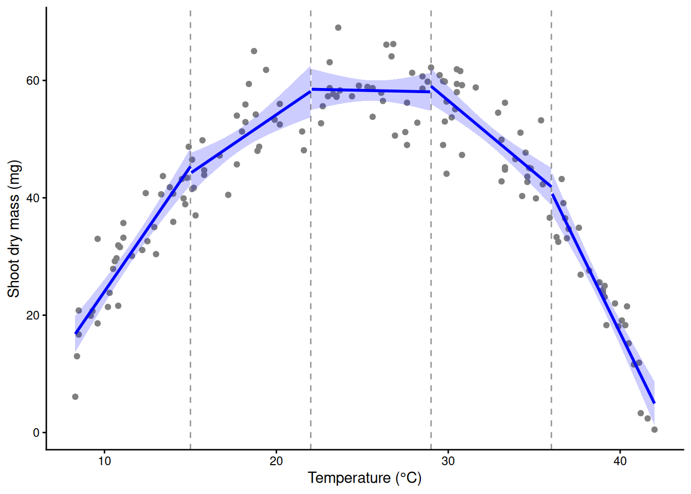

A spline joins the pieces: each is a small cubic, and neighbours meet with the same height, slope and curvature.

10) The basis: bumps, weights, and their sum

bs(temp, df = 6) makes six new columns. Each is a bump that is non-zero over one stretch of temperature. lm() gives each a coefficient; the weighted bumps, added up (plus the intercept), are the curve.

library(splines)
X <- bs(std$temp, df = 6)
round(head(X), 2)                 # one row per pot; most entries are 0

        1    2    3    4    5 6
[1,] 0.61 0.32 0.03 0.00 0.00 0
[2,] 0.00 0.05 0.56 0.38 0.00 0
[3,] 0.39 0.51 0.10 0.00 0.00 0
[4,] 0.51 0.42 0.06 0.00 0.00 0
[5,] 0.00 0.05 0.54 0.40 0.01 0
[6,] 0.58 0.10 0.00 0.00 0.00 0

m_bs <- lm(mass_mg ~ bs(temp, df = 6), data = std)
round(coef(m_bs), 1)              # intercept + one weight per bump

      (Intercept) bs(temp, df = 6)1 bs(temp, df = 6)2 bs(temp, df = 6)3 
             14.1              16.4              36.5              49.0 
bs(temp, df = 6)4 bs(temp, df = 6)5 bs(temp, df = 6)6 
             37.7              10.9             -12.4

summary(m_bs)$r.squared

[1] 0.9161993

ggplot(std, aes(temp, mass_mg)) +
  geom_point(colour = "grey50") +
  geom_ribbon(data = fit_ci(m_bs, grid), aes(temp, ymin = lwr, ymax = upr),
              inherit.aes = FALSE, fill = "blue", alpha = 0.2) +
  geom_line(data = fit_ci(m_bs, grid), aes(temp, fit), colour = "blue", linewidth = 1) +
  labs(x = "Temperature (°C)", y = "Shoot dry mass (mg)") +
  theme_classic()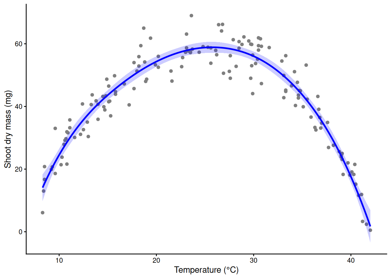

Demo: the weighted bumps and their sum

Xg <- predict(X, grid$temp)                # the same six columns on the grid
w <- coef(m_bs)
bumps <- data.frame(temp = rep(grid$temp, 6), value = as.vector(sweep(Xg, 2, w[-1], "*")),
                    bump = factor(rep(1:6, each = nrow(grid))))
total <- data.frame(temp = grid$temp, fit = w[1] + as.vector(Xg %*% w[-1]))
ggplot(std, aes(temp, mass_mg)) +
  geom_point(colour = "grey80") +
  geom_line(data = bumps, aes(temp, value, colour = bump), linewidth = 0.8) +
  geom_line(data = total, aes(temp, fit), colour = "black", linewidth = 1.3) +
  labs(x = "Temperature (°C)", y = "Weighted bump, and their sum (mg)") +
  theme_classic() + theme(legend.position = "none")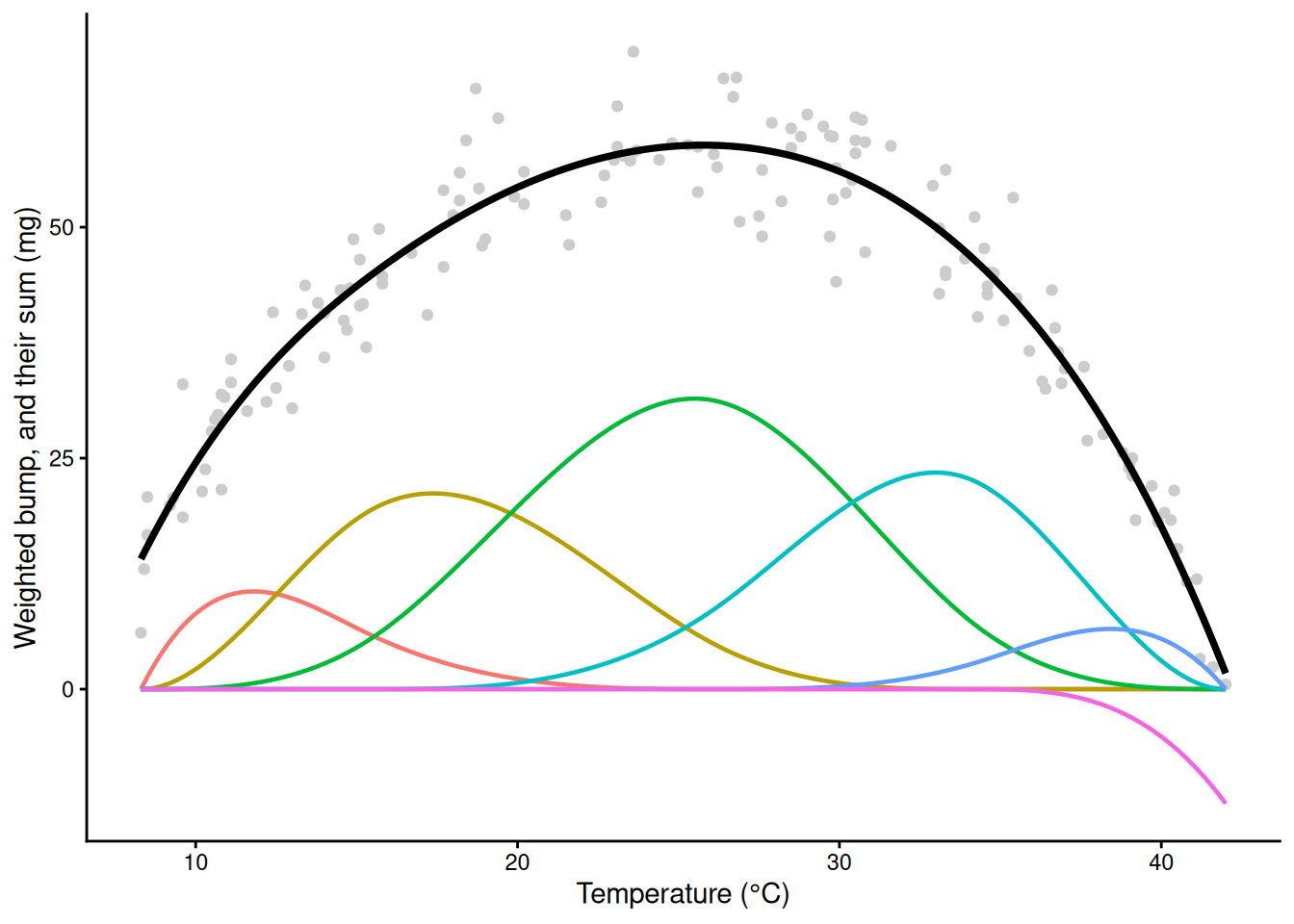

Demo: the weighted bumps and their sum

all.equal(total$fit, as.numeric(predict(m_bs, grid)))   # the sum is the fitted curve

[1] TRUE

Natural splines, ns(). The same idea, with one extra rule: beyond the outer knots the curve must be a straight line. Inside the data it fits like bs(); outside it stops bending. Because it is just columns in a formula, it drops into glm(), lmer() or any other model that takes a formula, which is how most applied papers add a curve for a covariate.

m_ns <- lm(mass_mg ~ ns(temp, df = 6), data = std)
summary(m_ns)$r.squared

[1] 0.9145374

wide <- data.frame(temp = seq(0, 50, length.out = 300))   # past the data on both sides
ggplot(std, aes(temp, mass_mg)) +
  geom_point(colour = "grey50") +
  geom_ribbon(data = fit_ci(m_ns, wide), aes(temp, ymin = lwr, ymax = upr),
              inherit.aes = FALSE, fill = "blue", alpha = 0.2) +
  geom_line(data = fit_ci(m_ns, wide), aes(temp, fit), colour = "blue", linewidth = 1) +
  geom_vline(xintercept = range(std$temp), linetype = 2) +    # the data stop here
  labs(x = "Temperature (°C)", y = "Shoot dry mass (mg)") +
  theme_classic()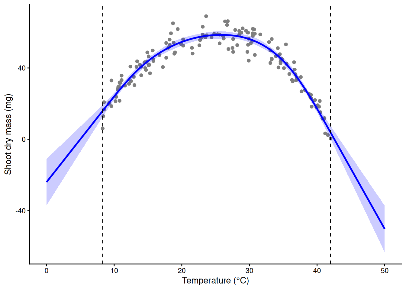

# outside the data: bs() keeps bending, ns() goes straight (both are still guesses there)
edges <- data.frame(temp = c(4, 46))
cbind(edges, bs = predict(m_bs, edges), ns = predict(m_ns, edges))

  temp        bs         ns
1    4 -26.27851  -4.746602
2   46 -42.03365 -23.195204

11) How many knots?

Too few columns and the curve is stiff; too many and it chases the noise.

fits <- list("2 straight pieces" = lm(mass_mg ~ bs(temp, df = 2, degree = 1), data = std),
             "df = 6"  = lm(mass_mg ~ bs(temp, df = 6), data = std),
             "df = 20" = lm(mass_mg ~ bs(temp, df = 20), data = std),
             "df = 40" = lm(mass_mg ~ bs(temp, df = 40), data = std))
sapply(fits, function(m) summary(m)$r.squared)

2 straight pieces            df = 6           df = 20           df = 40 
        0.8343224         0.9161993         0.9259303         0.9382672

ci_df <- do.call(rbind, lapply(names(fits), function(n) cbind(fit_ci(fits[[n]], grid), model = n)))
ci_df$model <- factor(ci_df$model, levels = names(fits))
ggplot(std, aes(temp, mass_mg)) +
  geom_point(colour = "grey60", size = 0.8) +
  geom_ribbon(data = ci_df, aes(temp, ymin = lwr, ymax = upr), inherit.aes = FALSE, fill = "blue", alpha = 0.2) +
  geom_line(data = ci_df, aes(temp, fit), colour = "blue") +
  facet_wrap(~ model) +
  labs(x = "Temperature (°C)", y = "Shoot dry mass (mg)") +
  theme_classic()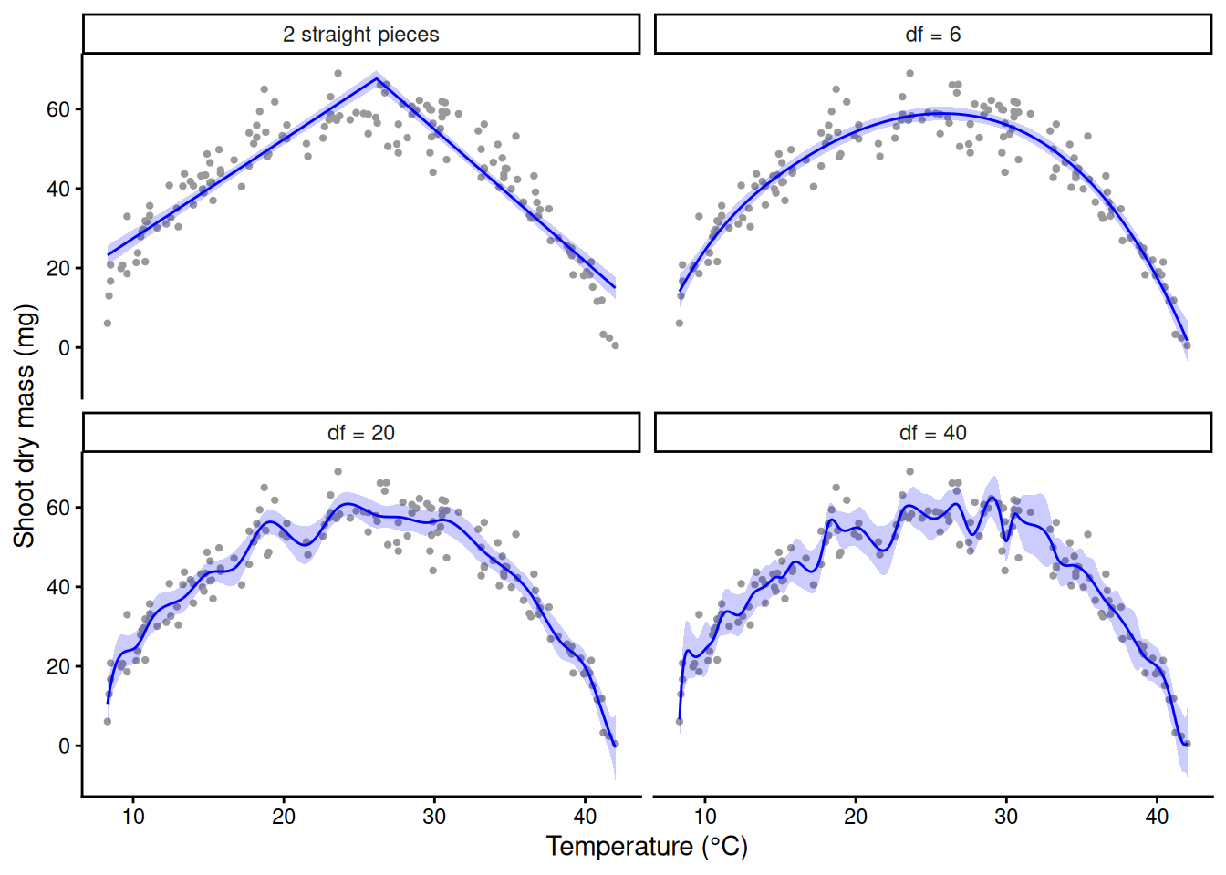

Picking this by eye is unsatisfying. A GAM lets the data choose (Part C).

12) Cycles: sin and cos columns

Soil respiration (CO₂ flux, µmol CO₂ m⁻² s⁻¹) on 8 permanent collars, every 14 days for two years. Simulated. Day of year is a circle: 31 December sits next to 1 January. A sine and a cosine of the day, as an angle around the year, are two new columns; a weighted sum of them is a wave with any height and timing that meets itself at the year’s end (a Fourier term).

soil <- read.csv("https://greymonroe.github.io/PLS_206/data/soil_season.csv")
head(soil)

  collar year day flux
1     C1 2024   5 1.29
2     C2 2024   5 2.22
3     C3 2024   5 1.08
4     C4 2024   5 1.65
5     C5 2024   5 1.67
6     C6 2024   5 1.07

f1 <- lm(flux ~ sin(2 * pi * day / 365) + cos(2 * pi * day / 365), data = soil)
f2 <- lm(flux ~ sin(2 * pi * day / 365) + cos(2 * pi * day / 365) +
                sin(4 * pi * day / 365) + cos(4 * pi * day / 365), data = soil)   # a second harmonic
c(one = summary(f1)$r.squared, two = summary(f2)$r.squared)

      one       two 
0.5950217 0.7281343

anova(f1, f2)    # the second pair of columns is needed

Analysis of Variance Table

Model 1: flux ~ sin(2 * pi * day/365) + cos(2 * pi * day/365)
Model 2: flux ~ sin(2 * pi * day/365) + cos(2 * pi * day/365) + sin(4 * 
    pi * day/365) + cos(4 * pi * day/365)
  Res.Df    RSS Df Sum of Sq      F    Pr(>F)    
1    413 235.49                                  
2    411 158.09  2    77.404 100.62 < 2.2e-16 ***
---
Signif. codes:  0 '***' 0.001 '**' 0.01 '*' 0.05 '.' 0.1 ' ' 1

g_day <- data.frame(day = 1:365)
four <- rbind(cbind(fit_ci(f1, g_day), model = "1 harmonic"), cbind(fit_ci(f2, g_day), model = "2 harmonics"))
ggplot(soil, aes(day, flux)) +
  geom_point(colour = "grey60", size = 0.8) +
  geom_ribbon(data = four, aes(day, ymin = lwr, ymax = upr), inherit.aes = FALSE, fill = "blue", alpha = 0.2) +
  geom_line(data = four, aes(day, fit), colour = "blue", linewidth = 1) +
  facet_wrap(~ model) +
  labs(x = "Day of year", y = expression(CO[2]~flux~(mu*mol~m^-2~s^-1))) +
  theme_classic()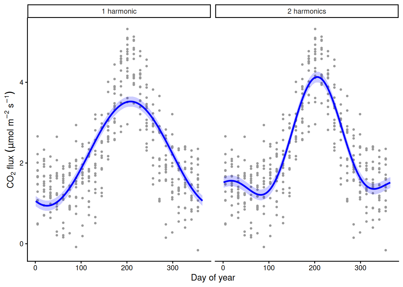

One sine–cosine pair is a symmetric wave and misses the fast spring rise and slow autumn decline; the second pair lets it lean.

13) loess: what geom_smooth draws

Reference. geom_smooth() (for fewer than 1000 points) draws a loess curve: a small weighted regression around every point, using its neighbours. Good for looking at data; it gives no model to summarise, test or report.

ggplot(std, aes(temp, mass_mg)) +
  geom_point(colour = "grey50") +
  geom_smooth() +                                   # method = "loess", span = 0.75
  labs(x = "Temperature (°C)", y = "Shoot dry mass (mg)") +
  theme_classic()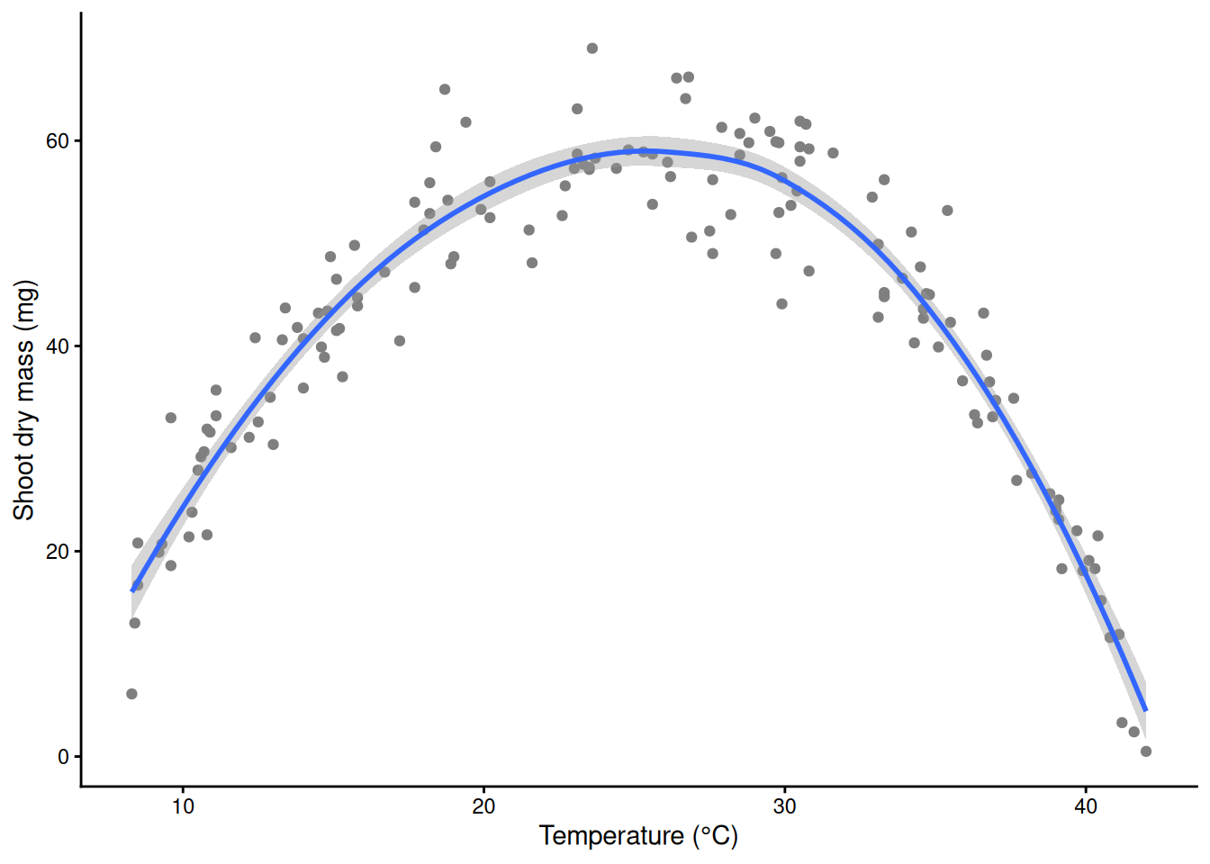

m_lo <- loess(mass_mg ~ temp, data = std)
m_lo                                                # "equivalent number of parameters"

Call:
loess(formula = mass_mg ~ temp, data = std)

Number of Observations: 150 
Equivalent Number of Parameters: 4.21 
Residual Standard Error: 4.6

Part C. GAMs

14) A penalized spline: lambda and edf

Give the spline many bumps (here 20) and add a penalty: minimise Σ(yᵢ − f(xᵢ))² + λ∫f’’(x)²dx. The first term fits the data; the second is the total curvature of the curve f, priced by λ. In gam(), sp = fixes λ by hand; normally the data choose it. bs = "bs" uses the B-spline bumps from Part B (the default s() uses a different set of columns; see section 18).

Demo: 20 basis functions with lambda tiny, chosen by REML, and huge

m_small <- gam(mass_mg ~ s(temp, bs = "bs", k = 20), data = std, sp = 1e-6, method = "REML")
m_reml  <- gam(mass_mg ~ s(temp, bs = "bs", k = 20), data = std, method = "REML")
m_huge  <- gam(mass_mg ~ s(temp, bs = "bs", k = 20), data = std, sp = 1e8, method = "REML")
pen <- list("lambda tiny" = m_small, "lambda chosen by REML" = m_reml, "lambda huge" = m_huge)
sapply(pen, function(m) c(lambda = m$full.sp[[1]], edf = sum(m$edf) - 1))   # edf of the smooth

       lambda tiny lambda chosen by REML  lambda huge
lambda    0.000001             17.435637 1.000000e+08
edf      18.999968              7.646988 1.000105e+00

Demo: 20 basis functions with lambda tiny, chosen by REML, and huge

cp <- do.call(rbind, lapply(names(pen), function(n) cbind(fit_ci(pen[[n]], grid), model = n)))
cp$model <- factor(cp$model, levels = names(pen))
ggplot(std, aes(temp, mass_mg)) +
  geom_point(colour = "grey75", size = 0.8) +
  geom_ribbon(data = cp, aes(temp, ymin = lwr, ymax = upr), inherit.aes = FALSE, fill = "black", alpha = 0.2) +
  geom_line(data = cp, aes(temp, fit), linewidth = 1.1) +
  facet_wrap(~ model) +
  coord_cartesian(ylim = c(-10, 80)) +
  labs(x = "Temperature (°C)", y = "Shoot dry mass (mg)") +
  theme_classic()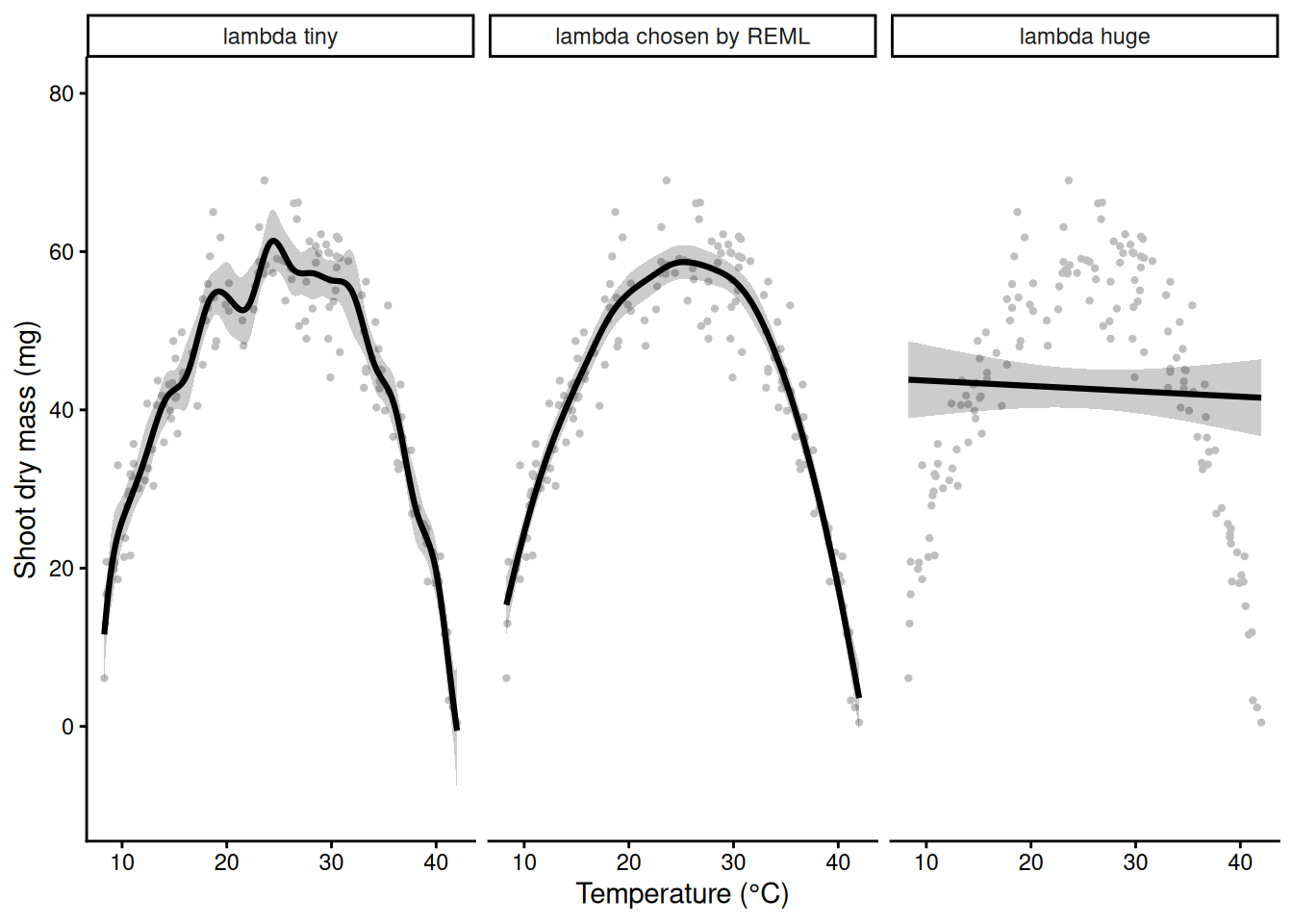

λ tiny: wiggles are free, edf about 19 (20 bumps minus one, lost to centring the smooth so that the intercept carries the overall level). λ huge: any bend is too expensive, and the curve becomes a straight line (edf = 1); the penalty never forbids a straight line. In between, edf (effective degrees of freedom) measures how many parameters the penalized curve is worth.

Demo: the penalty shrinks the bump weights; edf falls as lambda rises

wts <- do.call(rbind, lapply(names(pen), function(n)
  data.frame(bump = 1:19, weight = coef(pen[[n]])[-1], model = factor(n, levels = names(pen)))))
ggplot(wts, aes(bump, weight)) +
  geom_col(fill = "steelblue") +
  facet_wrap(~ model, scales = "free_y") +
  labs(x = "Basis function", y = "Coefficient") +
  theme_classic()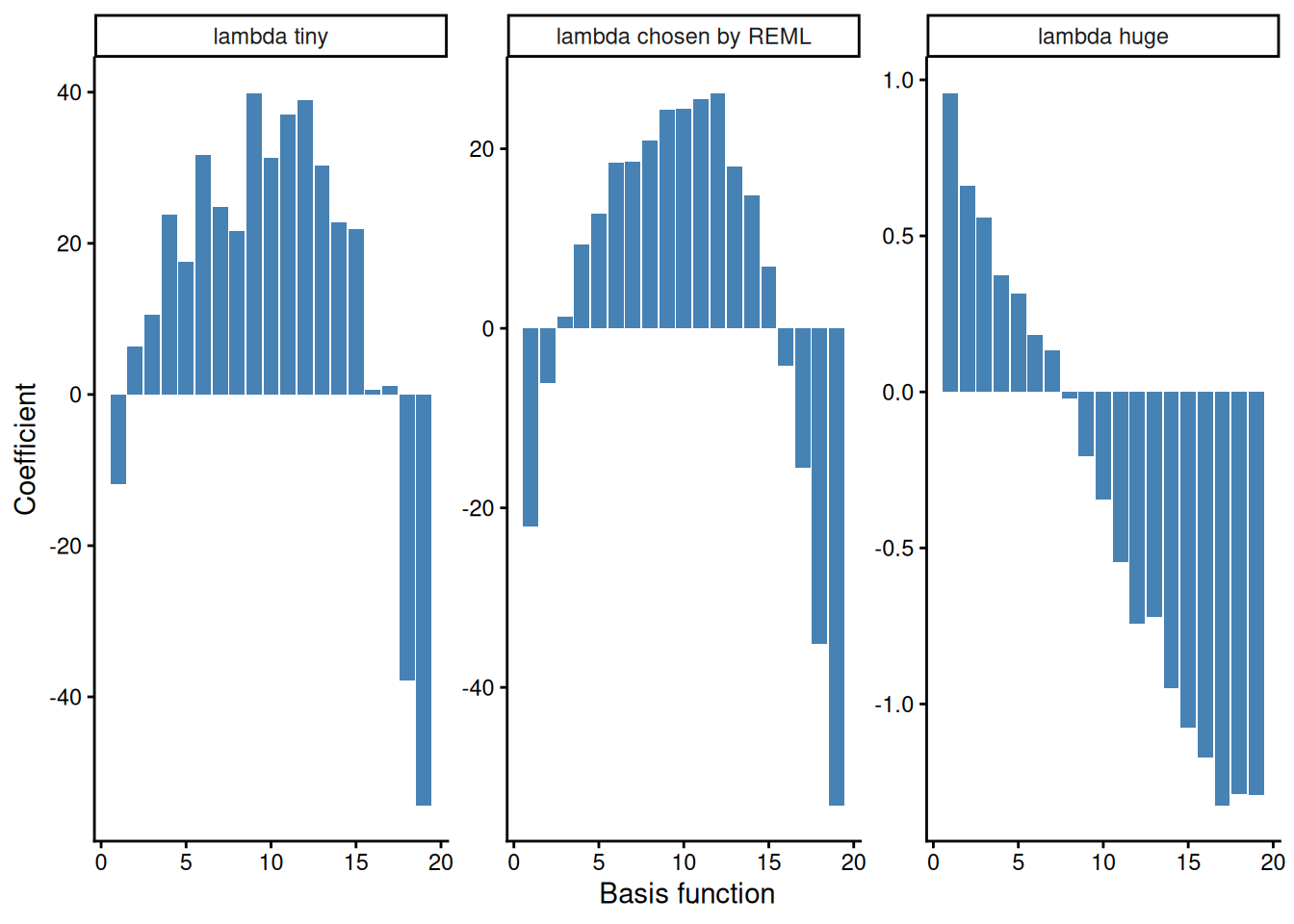

Demo: the penalty shrinks the bump weights; edf falls as lambda rises

lams <- 10^seq(-6, 8, by = 0.25)
edf_path <- sapply(lams, function(l) sum(gam(mass_mg ~ s(temp, bs = "bs", k = 20), data = std, sp = l)$edf) - 1)
ggplot(data.frame(log10_lambda = log10(lams), edf = edf_path), aes(log10_lambda, edf)) +
  geom_line(linewidth = 1) +
  geom_hline(yintercept = c(1, 19), linetype = 3) +
  geom_vline(xintercept = log10(m_reml$sp), colour = "red", linetype = 2) +
  labs(x = expression(log[10]~lambda), y = "edf of the smooth") +
  theme_classic()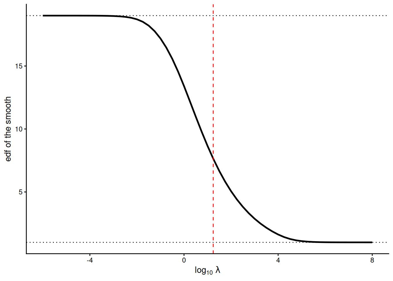

15) REML picks lambda

gam() tries values of λ and scores each. With method = "REML" the score is the restricted likelihood criterion, and gam() picks the λ at the bottom. mgcv’s default (GCV.Cp) usually gives a similar curve (here a slightly smoother one: edf 5.7 instead of 6.9, section 19), but it is more prone to occasionally picking a curve that is far too wiggly: always write method = "REML".

Demo: the REML score over a grid of lambda

lams <- 10^seq(-2, 7, by = 0.1)
score <- sapply(lams, function(l)
  gam(mass_mg ~ s(temp, bs = "bs", k = 20), data = std, sp = l, method = "REML")$gcv.ubre)
ggplot(data.frame(log10_lambda = log10(lams), REML = score), aes(log10_lambda, REML)) +
  geom_line(linewidth = 1) +
  geom_vline(xintercept = log10(m_reml$sp), colour = "red", linetype = 2) +
  labs(x = expression(log[10]~lambda), y = "REML score (lower is better)") +
  theme_classic()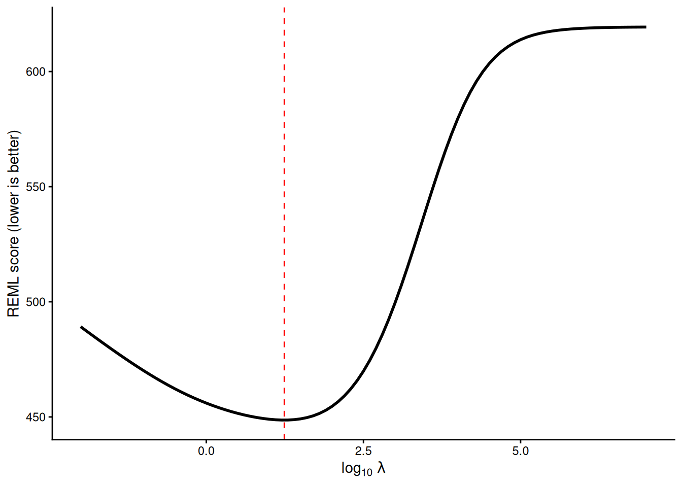

Demo: the REML score over a grid of lambda

m_reml$sp                       # the lambda REML chose

 s(temp) 
17.43564

16) Bias and variance

Simulate 30 new experiments from the true curve and fit each one. A tiny λ gives a different wiggle every time (variance); a huge λ gives the same wrong line every time (bias); REML lands near the truth.

Demo: 30 simulated experiments under three lambdas

beta_ct <- function(T, Tmin, Topt, Tmax) {     # the true growth curve used to simulate the data
  out <- ((Tmax - T) / (Tmax - Topt)) * ((T - Tmin) / (Topt - Tmin))^((Topt - Tmin) / (Tmax - Topt))
  ifelse(T > Tmin & T < Tmax, out, 0)
}
truth <- data.frame(temp = grid$temp, mass = 4 + 56 * beta_ct(grid$temp, 2, 26, 42))
set.seed(206)
reps <- do.call(rbind, lapply(1:30, function(r) {
  sim <- data.frame(temp = runif(150, 8, 42))
  sim$mass_mg <- pmax(0.5, 4 + 56 * beta_ct(sim$temp, 2, 26, 42) + rnorm(150, 0, 5))
  rbind(
    data.frame(temp = grid$temp, rep = r, model = "lambda tiny",
               fit = as.numeric(predict(gam(mass_mg ~ s(temp, bs = "bs", k = 20), data = sim, sp = 1e-6), grid))),
    data.frame(temp = grid$temp, rep = r, model = "lambda chosen by REML",
               fit = as.numeric(predict(gam(mass_mg ~ s(temp, bs = "bs", k = 20), data = sim, method = "REML"), grid))),
    data.frame(temp = grid$temp, rep = r, model = "lambda huge",
               fit = as.numeric(predict(gam(mass_mg ~ s(temp, bs = "bs", k = 20), data = sim, sp = 1e8), grid))))
}))
reps$model <- factor(reps$model, levels = names(pen))
ggplot(reps, aes(temp, fit, group = rep)) +
  geom_line(colour = "grey40", alpha = 0.4) +
  geom_line(data = truth, aes(temp, mass), inherit.aes = FALSE, colour = "red", linetype = 2, linewidth = 1) +
  facet_wrap(~ model) +
  coord_cartesian(ylim = c(-10, 80)) +
  labs(x = "Temperature (°C)", y = "Fitted shoot mass (mg)") +
  theme_classic()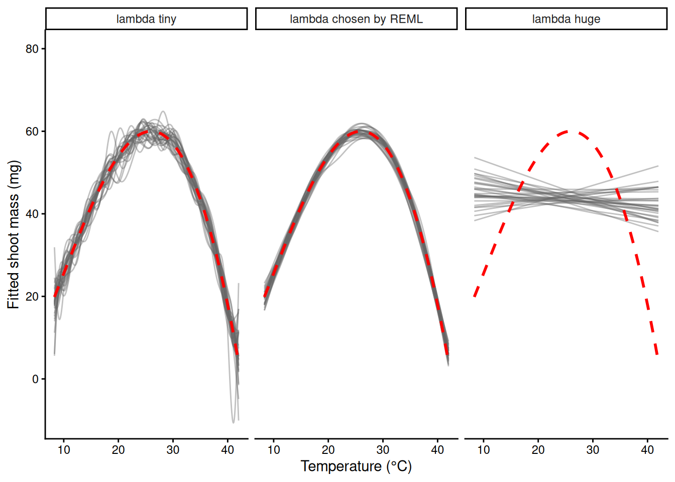

The same penalty idea comes back in Week 6 as ridge regression: Σ(y − ŷ)² + λΣβⱼ², shrinking ordinary regression coefficients with a λ chosen from the data.

17) k is a ceiling

In s(temp, k = ...), k sets the number of basis functions: the maximum wiggliness. The penalty decides the actual wiggliness. Once k is big enough, more bumps give the same curve.

ks <- c(5, 10, 20, 40)
m_k <- lapply(ks, function(k) gam(mass_mg ~ s(temp, k = k), data = std, method = "REML"))
names(m_k) <- paste("k =", ks)
sapply(m_k, function(m) sum(m$edf) - 1)    # edf: about 4, 6.9, 7.8, 7.9

   k = 5   k = 10   k = 20   k = 40 
3.954184 6.869345 7.753768 7.851280

ck <- do.call(rbind, lapply(names(m_k), function(n) cbind(fit_ci(m_k[[n]], grid), model = n)))
ck$model <- factor(ck$model, levels = names(m_k))
ggplot(std, aes(temp, mass_mg)) +
  geom_point(colour = "grey70") +
  geom_ribbon(data = ck, aes(temp, ymin = lwr, ymax = upr, fill = model), inherit.aes = FALSE, alpha = 0.1) +
  geom_line(data = ck, aes(temp, fit, colour = model), linewidth = 1) +
  labs(x = "Temperature (°C)", y = "Shoot dry mass (mg)", colour = NULL, fill = NULL) +
  theme_classic()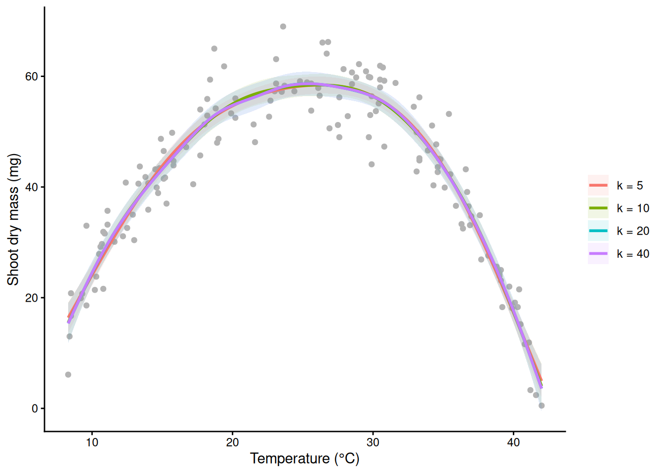

18) Your first GAM

m_gam <- gam(mass_mg ~ s(temp), data = std, method = "REML")   # thin-plate smooth, k = 10 by default
ci_gam <- fit_ci(m_gam, grid)
opt <- ci_gam$temp[which.max(ci_gam$fit)]
opt                                                            # the fitted optimum: 26.25 °C

[1] 26.25

ggplot(std, aes(temp, mass_mg)) +
  geom_point(colour = "grey50") +
  geom_ribbon(data = ci_gam, aes(temp, ymin = lwr, ymax = upr), inherit.aes = FALSE, fill = "blue", alpha = 0.2) +
  geom_line(data = ci_gam, aes(temp, fit), colour = "blue", linewidth = 1) +
  geom_vline(xintercept = opt, colour = "red", linetype = 2) +
  labs(x = "Temperature (°C)", y = "Shoot dry mass (mg)") +
  theme_classic()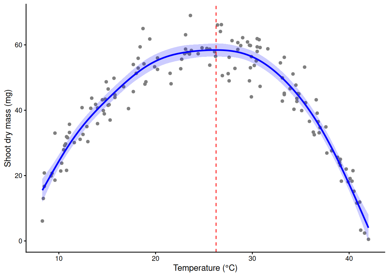

The GAM finds the slow rise and the cliff, and its peak lands near the true 26 °C that the parabola (24.6 °C) missed.

Part D. Reading a GAM

19) The summary, line by line

summary(m_gam)


Family: gaussian 
Link function: identity 

Formula:
mass_mg ~ s(temp)

Parametric coefficients:
            Estimate Std. Error t value Pr(>|t|)    
(Intercept)  42.6800     0.3765   113.4   <2e-16 ***
---
Signif. codes:  0 '***' 0.001 '**' 0.01 '*' 0.05 '.' 0.1 ' ' 1

Approximate significance of smooth terms:
          edf Ref.df     F p-value    
s(temp) 6.869   7.98 192.4  <2e-16 ***
---
Signif. codes:  0 '***' 0.001 '**' 0.01 '*' 0.05 '.' 0.1 ' ' 1

R-sq.(adj) =  0.912   Deviance explained = 91.6%
-REML =  450.4  Scale est. = 21.261    n = 150

mean(std$mass_mg)   # the same number as the intercept

[1] 42.68

Walking down it:

Family / Link function / Formula. Gaussian with an identity link: ordinary normal errors, as in lm(). A GAM takes any family from Week 3 (binomial, Poisson, …) with its link: a GAM is a GLM whose linear predictor can contain curves.
Parametric coefficients. Only an intercept, and it equals mean(std$mass_mg), not the mass at 0 °C. mgcv centres every smooth so that it sums (averages) to zero over the data, so all the shape lives in the smooth and the intercept sets the overall level. Its SE is the uncertainty in that mean.
edf. Effective degrees of freedom of the smooth: how many parameters of bend the penalty allowed. 1 = a straight line; about 2 = roughly a quadratic; the maximum is k − 1 (9 for the default k = 10). Near 1: a straight line would have done. Near k − 1: check k (section 21).
Ref.df, F, p-value. A test of one question: is the smooth flat (zero everywhere)? Ref.df is the reference degrees of freedom used for that test. The p-value is approximate, because the penalty makes exact theory hard: treat values near 0.05 with suspicion.
R-sq.(adj). Adjusted R², as in lm().
Deviance explained. The version that works for every family; for a Gaussian model it equals the unadjusted R². Report this for binomial and Poisson GAMs.
-REML. The REML score at the chosen λ (the bottom of the curve in section 15). Only useful for comparing models fitted to the same data.
Scale est. The residual variance; its square root is the typical scatter of a pot around the curve, in mg.
n. The number of observations (150 pots).

sqrt(m_gam$sig2)                                  # residual SD, mg

[1] 4.610968

m_gcv <- gam(mass_mg ~ s(temp), data = std)       # mgcv's default method (GCV.Cp)
c(REML = sum(m_gam$edf) - 1, GCV = sum(m_gcv$edf) - 1)   # different edf: say which you used

    REML      GCV 
6.869345 5.734285

20) Partial-effect plots

plot() on a GAM draws each smooth on its own: the partial effect, centred at zero (the intercept is not included), on the link scale, with a ±2 SE band and a rug showing where the data are. The y-axis label includes the edf.

plot(m_gam, shade = TRUE, rug = TRUE)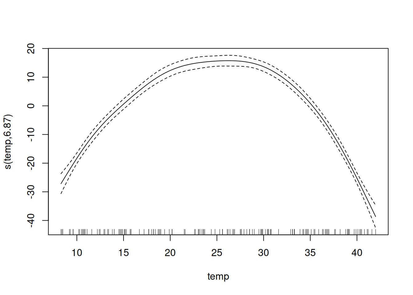

Demo: the centred smooth plus the intercept is the fitted curve

pt <- predict(m_gam, grid, type = "terms", se.fit = TRUE)
part <- data.frame(temp = grid$temp, s = pt$fit[, 1], se = pt$se.fit[, 1])
range(part$s)                              # above and below zero

[1] -38.64961  15.75155

Demo: the centred smooth plus the intercept is the fitted curve

mean(predict(m_gam, type = "terms"))       # averages zero over the data

[1] -5.215492e-15

Demo: the centred smooth plus the intercept is the fitted curve

all.equal(as.numeric(part$s + coef(m_gam)[1]), as.numeric(predict(m_gam, grid)))

[1] TRUE

For a figure, put the curve back on the scale of y with the data underneath (fit_ci() from section 3). That is the figure from section 18; with several smooths in a model, predict over a grid of one predictor while holding the others at typical values.

21) Is k big enough?

gam.check() prints a k check and draws four residual panels (QQ plot, residuals vs linear predictor, histogram, response vs fitted: the Week 2 checks). k.check() prints just the k check. Its p-value comes from a random permutation test, so set a seed to get the same p-value twice.

set.seed(206)
gam.check(m_gam)            # k-index 0.95, p well above 0.05, edf 6.9 of k' = 9: fine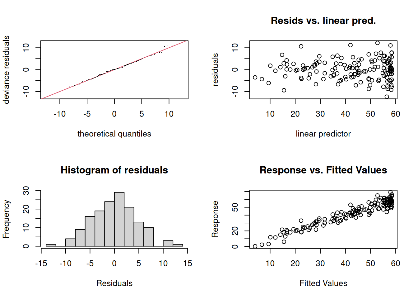


Method: REML   Optimizer: outer newton
full convergence after 6 iterations.
Gradient range [-2.728313e-05,2.355657e-05]
(score 450.3975 & scale 21.26102).
Hessian positive definite, eigenvalue range [2.699505,74.12082].
Model rank =  10 / 10 

Basis dimension (k) checking results. Low p-value (k-index<1) may
indicate that k is too low, especially if edf is close to k'.

          k'  edf k-index p-value
s(temp) 9.00 6.87    0.95    0.28

Now a deliberately small k:

m4  <- gam(mass_mg ~ s(temp, k = 4),  data = std, method = "REML")
m8  <- gam(mass_mg ~ s(temp, k = 8),  data = std, method = "REML")
m16 <- gam(mass_mg ~ s(temp, k = 16), data = std, method = "REML")
set.seed(206); k.check(m4)    # k-index < 1, small p, edf pressed against k' = 3: too small

        k'      edf   k-index p-value
s(temp)  3 2.987211 0.7854077  0.0025

set.seed(206); k.check(m8)    # double k: passes

        k'      edf   k-index p-value
s(temp)  7 6.056363 0.9335162  0.2025

set.seed(206); k.check(m16)   # double again

        k'      edf   k-index p-value
s(temp) 15 7.617236 0.9618221  0.3225

The rule: if the k-index is below 1 with a small p-value and the edf is close to k’, double k and refit. If the curve barely changes, the old k was fine (and a low k-index may come from something else, like correlated residuals). If it changes, double again. The test is the curve, not the edf:

g941 <- data.frame(temp = seq(9, 41, by = 0.1))
max(abs(predict(m8, g941) - predict(m16, g941)))   # k = 8 vs 16: under 1 mg apart anywhere

[1] 0.6124941

max(abs(predict(m4, g941) - predict(m16, g941)))   # k = 4 vs 16: more than 3 mg apart

[1] 3.177773

c48 <- do.call(rbind, lapply(list(`k = 4` = m4, `k = 8` = m8, `k = 16` = m16), function(m) fit_ci(m, grid)))
c48$model <- rep(c("k = 4", "k = 8", "k = 16"), each = nrow(grid))
ggplot(std, aes(temp, mass_mg)) +
  geom_point(colour = "grey70") +
  geom_ribbon(data = c48, aes(temp, ymin = lwr, ymax = upr, fill = model), inherit.aes = FALSE, alpha = 0.12) +
  geom_line(data = c48, aes(temp, fit, colour = model), linewidth = 1) +
  labs(x = "Temperature (°C)", y = "Shoot dry mass (mg)", colour = NULL, fill = NULL) +
  theme_classic()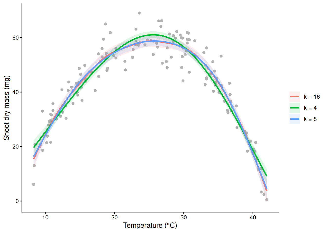

A GAM fixes the shape of the mean. It does not fix unequal spread, the wrong family, or non-independent observations: read the four residual panels as you would for lm().

22) Reporting a curve, and where it rises and falls

A curve has no single slope to quote. Show the figure, and report edf, F (or χ² for non-Gaussian families), the p-value and the deviance explained. To say where the response rises or falls, take the derivative of the fitted curve with a confidence band: gratia::derivatives(). A simultaneous interval covers the whole curve at once.

# install.packages("gratia")
library(gratia)
d <- derivatives(m_gam, select = "s(temp)", interval = "simultaneous", n = 200)
d$trend <- ifelse(d$.lower_ci > 0, "rising", ifelse(d$.upper_ci < 0, "falling", "not distinguishable from flat"))
ci_d <- fit_ci(m_gam, data.frame(temp = d$temp))
ci_d$trend <- d$trend
ggplot(std, aes(temp, mass_mg)) +
  geom_point(colour = "grey75") +
  geom_ribbon(data = ci_d, aes(temp, ymin = lwr, ymax = upr), inherit.aes = FALSE, fill = "grey60", alpha = 0.3) +
  geom_line(data = ci_d, aes(temp, fit, colour = trend, group = 1), linewidth = 1.5) +
  scale_colour_manual(values = c(rising = "blue", falling = "red", "not distinguishable from flat" = "grey40")) +
  labs(x = "Temperature (°C)", y = "Shoot dry mass (mg)", colour = NULL) +
  theme_classic() + theme(legend.position = "top")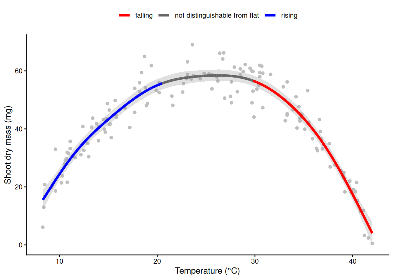

range(d$temp[d$trend == "not distinguishable from flat"])   # the plateau around the optimum

[1] 20.49296 29.63769

Example sentences:

Methods. Shoot mass was modelled as a smooth function of temperature with a generalized additive model (mgcv, REML smoothness selection, k = 10).
Results. Temperature had a strong non-linear effect on shoot mass (edf = 6.87, F = 192.4, p < 0.001; deviance explained 91.6%), peaking at about 26 °C (Fig. 1).

Part E. The GAM toolkit

23) Yes/no responses: a binomial GAM

The same pots: were the leaves damaged (chilling at the cold end, heat scorch at the hot end)? A logistic GLM is a straight line on the log-odds scale and cannot make a U.

m_dglm <- glm(damaged ~ temp, family = binomial, data = std)
round(coef(summary(m_dglm)), 3)     # slope p = 0.90: nothing, again

            Estimate Std. Error z value Pr(>|z|)
(Intercept)   -0.602      0.458  -1.314    0.189
temp           0.002      0.017   0.130    0.896

m_dmg <- gam(damaged ~ s(temp), family = binomial, data = std, method = "REML")
summary(m_dmg)                      # Chi.sq instead of F; report deviance explained


Family: binomial 
Link function: logit 

Formula:
damaged ~ s(temp)

Parametric coefficients:
            Estimate Std. Error z value Pr(>|z|)    
(Intercept)  -0.7303     0.2178  -3.353 0.000798 ***
---
Signif. codes:  0 '***' 0.001 '**' 0.01 '*' 0.05 '.' 0.1 ' ' 1

Approximate significance of smooth terms:
          edf Ref.df Chi.sq p-value    
s(temp) 3.471  4.303   38.8 1.1e-07 ***
---
Signif. codes:  0 '***' 0.001 '**' 0.01 '*' 0.05 '.' 0.1 ' ' 1

R-sq.(adj) =  0.335   Deviance explained = 28.7%
-REML = 75.359  Scale est. = 1         n = 150

plogis(predict(m_dmg, data.frame(temp = c(8, 25, 40))))   # P(damage) at 8, 25, 40 °C

         1          2          3 
0.86687666 0.07538283 0.82381283

plot(m_dmg) shows the smooth on the log-odds scale, centred at zero. For a figure on the probability scale, build the band on the link scale and convert the fit and both edges with plogis(); that keeps the band between 0 and 1. (fit_ci() does exactly this.)

p <- predict(m_dmg, grid, se.fit = TRUE)          # link (log-odds) scale
dmg_ci <- data.frame(temp = grid$temp,
                     fit = plogis(p$fit),
                     lwr = plogis(p$fit - 1.96 * p$se.fit),
                     upr = plogis(p$fit + 1.96 * p$se.fit))
dmg_glm_ci <- fit_ci(m_dglm, grid)
ggplot(std, aes(temp, damaged)) +
  geom_jitter(width = 0, height = 0.03, colour = "grey50") +
  geom_ribbon(data = dmg_glm_ci, aes(temp, ymin = lwr, ymax = upr), inherit.aes = FALSE, fill = "grey40", alpha = 0.2) +
  geom_line(data = dmg_glm_ci, aes(temp, fit), colour = "grey40", linetype = 2) +
  geom_ribbon(data = dmg_ci, aes(temp, ymin = lwr, ymax = upr), inherit.aes = FALSE, fill = "red", alpha = 0.2) +
  geom_line(data = dmg_ci, aes(temp, fit), colour = "red", linewidth = 1) +
  labs(x = "Temperature (°C)", y = "P(leaf damage)", subtitle = "dashed: logistic GLM; red: binomial GAM") +
  theme_classic()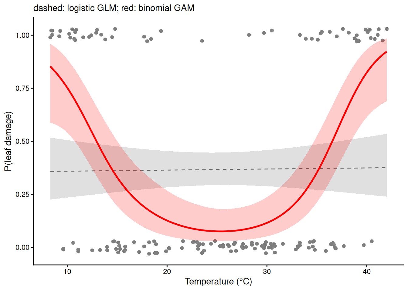

24) One curve per group: by =

Both varieties now. s(temp, by = variety) gives each variety its own smooth with its own wiggliness. Each by-smooth is centred at zero, so it describes shape only: the factor must also be in the model as a main effect to set each group’s level. by = needs a factor.

seedlings$variety <- factor(seedlings$variety)
m_by <- gam(mass_mg ~ variety + s(temp, by = variety), data = seedlings, method = "REML")
summary(m_by)     # varietytolerant: difference in average mass; one smooth row per variety


Family: gaussian 
Link function: identity 

Formula:
mass_mg ~ variety + s(temp, by = variety)

Parametric coefficients:
                Estimate Std. Error t value Pr(>|t|)    
(Intercept)      42.5874     0.3916 108.759  < 2e-16 ***
varietytolerant   1.8393     0.5535   3.323  0.00101 ** 
---
Signif. codes:  0 '***' 0.001 '**' 0.01 '*' 0.05 '.' 0.1 ' ' 1

Approximate significance of smooth terms:
                          edf Ref.df     F p-value    
s(temp):varietystandard 6.761  7.885 181.7  <2e-16 ***
s(temp):varietytolerant 5.473  6.609 116.6  <2e-16 ***
---
Signif. codes:  0 '***' 0.001 '**' 0.01 '*' 0.05 '.' 0.1 ' ' 1

R-sq.(adj) =  0.881   Deviance explained = 88.6%
-REML = 907.63  Scale est. = 22.777    n = 300

nd38 <- data.frame(temp = 38, variety = factor(c("standard", "tolerant"), levels = levels(seedlings$variety)))
fit_ci(m_by, nd38)   # at 38 °C the two CIs are far apart

  temp  variety      fit      lwr      upr
1   38 standard 29.55129 27.47039 31.63218
2   38 tolerant 45.55767 43.78663 47.32871

gv <- expand.grid(temp = seq(8, 42, by = 0.1), variety = levels(seedlings$variety))
ci_by <- fit_ci(m_by, gv)
ggplot(seedlings, aes(temp, mass_mg, colour = variety)) +
  geom_point(alpha = 0.5) +
  geom_ribbon(data = ci_by, aes(temp, ymin = lwr, ymax = upr, fill = variety), inherit.aes = FALSE, alpha = 0.2) +
  geom_line(data = ci_by, aes(temp, fit, colour = variety), linewidth = 1) +
  labs(x = "Temperature (°C)", y = "Shoot dry mass (mg)") +
  theme_classic()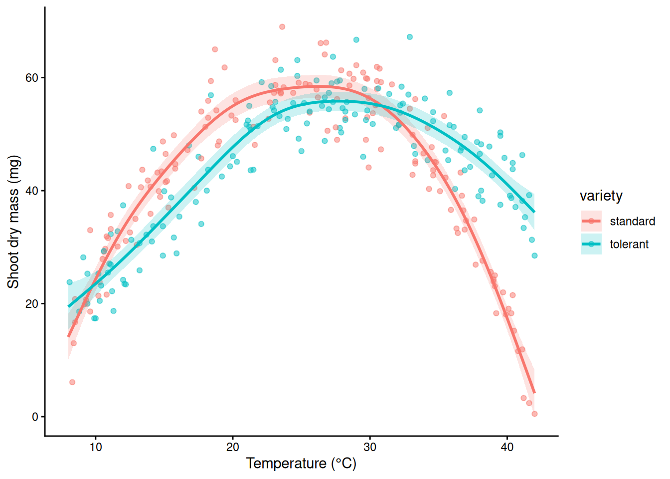

Demo: what goes wrong without the variety main effect

m_trap <- gam(mass_mg ~ s(temp, by = variety), data = seedlings, method = "REML")
ci_trap <- fit_ci(m_trap, gv)
tapply(predict(m_trap), seedlings$variety, mean)   # pulled to nearly the same average

standard tolerant 
43.59176 43.80024

Demo: what goes wrong without the variety main effect

tapply(seedlings$mass_mg, seedlings$variety, mean) # but the varieties' means differ

standard tolerant 
  42.680   44.712

Demo: what goes wrong without the variety main effect

ggplot(seedlings, aes(temp, mass_mg, colour = variety)) +
  geom_point(alpha = 0.4) +
  geom_ribbon(data = ci_trap, aes(temp, ymin = lwr, ymax = upr, fill = variety), inherit.aes = FALSE, alpha = 0.2) +
  geom_line(data = ci_trap, aes(temp, fit, colour = variety), linewidth = 1) +
  labs(x = "Temperature (°C)", y = "Shoot dry mass (mg)", title = "No variety main effect: wrong") +
  theme_classic()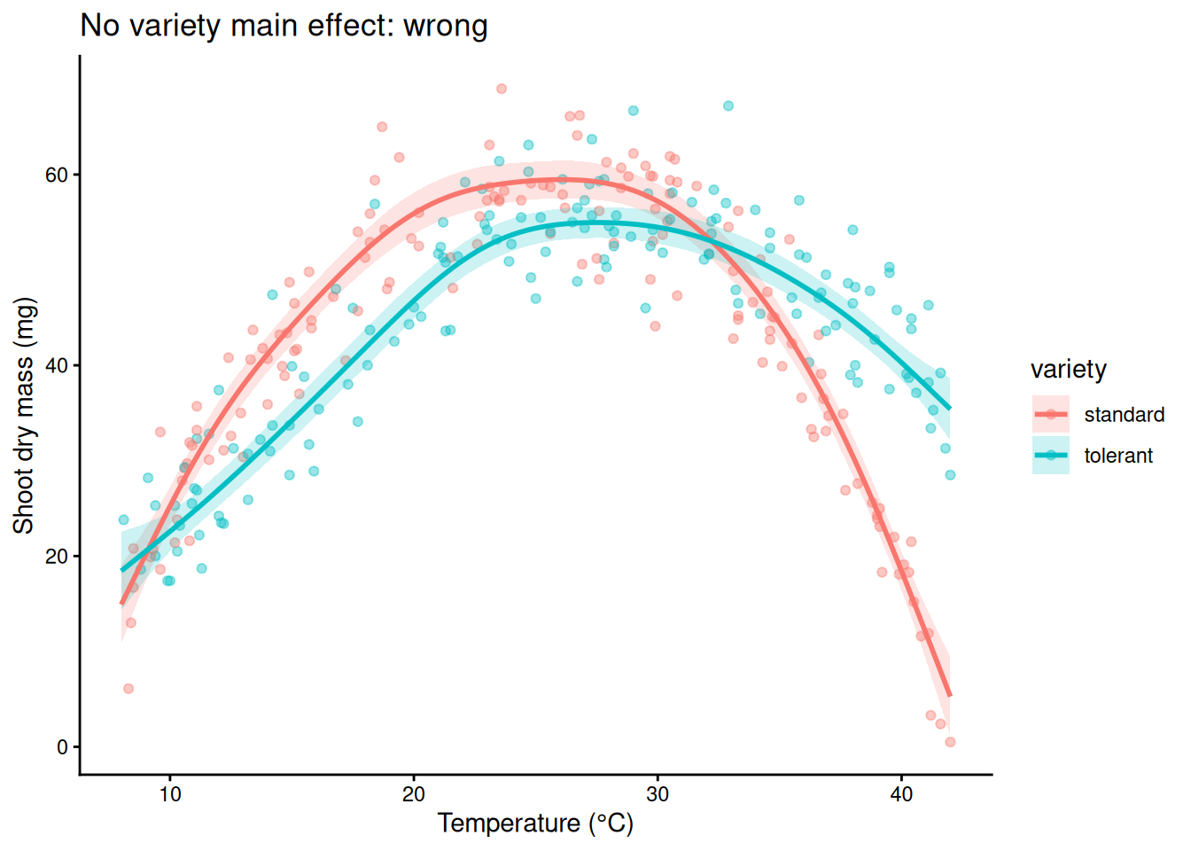

25) Cycles: bs = “cc”

An ordinary smooth of day does not know that day 365 is next to day 1, so its ends need not meet. A cyclic cubic spline, bs = "cc", forces the curve to join up smoothly: section 12’s Fourier idea in spline form. Put the end knots at the edges of the year so the join falls between 31 December and 1 January. Here k = 20: in the full model of section 26, k = 12 left the edf at 9.2 of a possible 10, pressing on its ceiling.

soil$collar <- factor(soil$collar)
m_tp <- gam(flux ~ s(day), data = soil, method = "REML")
m_cc <- gam(flux ~ s(day, bs = "cc", k = 20), data = soil, method = "REML",
            knots = list(day = c(0.5, 365.5)))
ends <- data.frame(day = c(0.5, 365.5))
predict(m_tp, ends)   # ordinary smooth: the ends don't match

       1        2 
1.602231 1.392230

predict(m_cc, ends)   # cyclic: identical

       1        2 
1.491093 1.491093

g_day <- data.frame(day = 1:365)
ci_ends <- rbind(cbind(fit_ci(m_tp, g_day), model = "s(day): ordinary"),
                 cbind(fit_ci(m_cc, g_day), model = "s(day, bs = \"cc\"): cyclic"))
ggplot(soil, aes(day, flux)) +
  geom_point(colour = "grey60", size = 0.8) +
  geom_ribbon(data = ci_ends, aes(day, ymin = lwr, ymax = upr), inherit.aes = FALSE, fill = "blue", alpha = 0.2) +
  geom_line(data = ci_ends, aes(day, fit), colour = "blue", linewidth = 1) +
  facet_wrap(~ model) +
  labs(x = "Day of year", y = expression(CO[2]~flux~(mu*mol~m^-2~s^-1))) +
  theme_classic()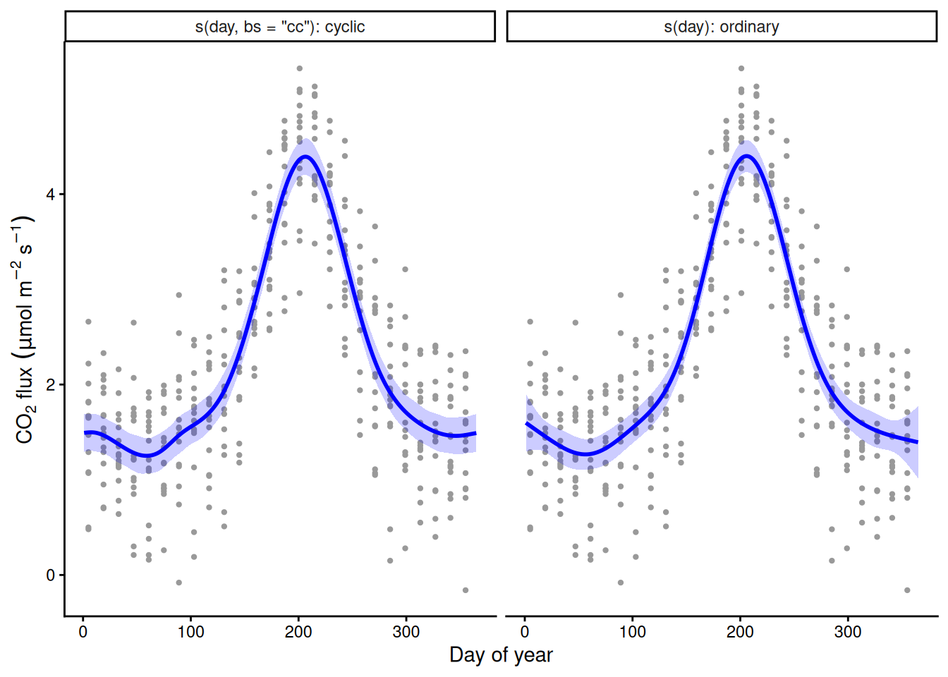

26) Random effects: bs = “re”

The eight collars differ in baseline respiration, and repeated measurements on one collar are not independent. s(collar, bs = "re") is a random intercept for each collar, the same as (1 | collar) in last week’s mixed models. collar must be a factor.

m_soil <- gam(flux ~ s(day, bs = "cc", k = 20) + s(collar, bs = "re"), data = soil,
              method = "REML", knots = list(day = c(0.5, 365.5)))
summary(m_soil)


Family: gaussian 
Link function: identity 

Formula:
flux ~ s(day, bs = "cc", k = 20) + s(collar, bs = "re")

Parametric coefficients:
            Estimate Std. Error t value Pr(>|t|)    
(Intercept)   2.2359     0.1801   12.42   <2e-16 ***
---
Signif. codes:  0 '***' 0.001 '**' 0.01 '*' 0.05 '.' 0.1 ' ' 1

Approximate significance of smooth terms:
             edf Ref.df     F p-value    
s(day)    12.104     18 187.7  <2e-16 ***
s(collar)  6.933      7 103.8  <2e-16 ***
---
Signif. codes:  0 '***' 0.001 '**' 0.01 '*' 0.05 '.' 0.1 ' ' 1

R-sq.(adj) =  0.908   Deviance explained = 91.2%
-REML = 203.77  Scale est. = 0.12865   n = 416

gam.vcomp(m_soil)     # the collar SD (true value 0.5) and the residual SD


Standard deviations and 0.95 confidence intervals:

              std.dev      lower       upper
s(day)    0.004405793 0.00298406 0.006504901
s(collar) 0.506844712 0.29866945 0.860119974
scale     0.358677533 0.33456006 0.384533560

Rank: 3/3

All smooth components:
[1] 0.004405793 0.506844712

set.seed(206); k.check(m_soil)

          k'       edf   k-index p-value
s(day)    18 12.103975 0.9883657  0.3375
s(collar)  8  6.933229        NA      NA

gd <- data.frame(day = 1:365, collar = factor("C1", levels = levels(soil$collar)))
ci_soil <- fit_ci(m_soil, gd)    # the seasonal curve for collar C1
ggplot(soil, aes(day, flux)) +
  geom_point(aes(colour = collar), size = 0.8, alpha = 0.6) +
  geom_ribbon(data = ci_soil, aes(day, ymin = lwr, ymax = upr), inherit.aes = FALSE, fill = "black", alpha = 0.2) +
  geom_line(data = ci_soil, aes(day, fit), linewidth = 1) +
  labs(x = "Day of year", y = expression(CO[2]~flux~(mu*mol~m^-2~s^-1)), title = "Seasonal curve for collar C1") +
  theme_classic()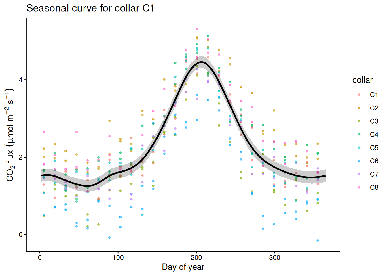

# each collar's estimated offset with a 95% CI
re_cols <- grep("s\\(collar\\)", names(coef(m_soil)))
offs <- data.frame(collar = levels(soil$collar), est = coef(m_soil)[re_cols],
                   se = sqrt(diag(vcov(m_soil)))[re_cols])
ggplot(offs, aes(collar, est)) +
  geom_hline(yintercept = 0, linetype = 2) +
  geom_pointrange(aes(ymin = est - 1.96 * se, ymax = est + 1.96 * se)) +
  labs(x = "Collar", y = "Offset from the average collar") +
  theme_classic()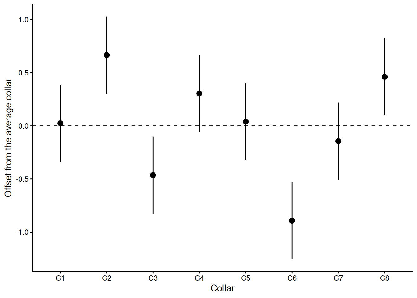

27) Field heterogeneity: s(x, y)

A rice trial: a gene-edited line vs its wild type, 100 plots of each, randomised over a 20 x 10 grid of 3 m plots. The field has an unrecorded fertility gradient. Simulated.

field <- read.csv("https://greymonroe.github.io/PLS_206/data/field_gradient.csv")
field$genotype <- factor(field$genotype, levels = c("wildtype", "edited"))
m_naive <- lm(yield ~ genotype, data = field)
round(coef(summary(m_naive)), 4)        # ignore the field: no detectable effect

               Estimate Std. Error t value Pr(>|t|)
(Intercept)       6.966     0.1174 59.3171   0.0000
genotypeedited    0.122     0.1661  0.7346   0.4635

m_sp <- gam(yield ~ genotype + s(x_m, y_m), data = field, method = "REML")
summary(m_sp)                           # model the field: the effect appears


Family: gaussian 
Link function: identity 

Formula:
yield ~ genotype + s(x_m, y_m)

Parametric coefficients:
               Estimate Std. Error t value Pr(>|t|)    
(Intercept)     6.90622    0.04242  162.79  < 2e-16 ***
genotypeedited  0.24156    0.06178    3.91 0.000132 ***
---
Signif. codes:  0 '***' 0.001 '**' 0.01 '*' 0.05 '.' 0.1 ' ' 1

Approximate significance of smooth terms:
             edf Ref.df     F p-value    
s(x_m,y_m) 21.39  25.87 54.56  <2e-16 ***
---
Signif. codes:  0 '***' 0.001 '**' 0.01 '*' 0.05 '.' 0.1 ' ' 1

R-sq.(adj) =  0.877   Deviance explained = 89.1%
-REML = 137.08  Scale est. = 0.16911   n = 200

ggplot(field, aes(x_m, y_m, fill = yield)) +
  geom_tile() +
  geom_point(aes(shape = genotype), colour = "white", size = 1.5) +
  scale_fill_viridis_c() +
  coord_fixed() +
  labs(x = "x (m)", y = "y (m)", fill = "Yield (t/ha)", title = "The field") +
  theme_classic()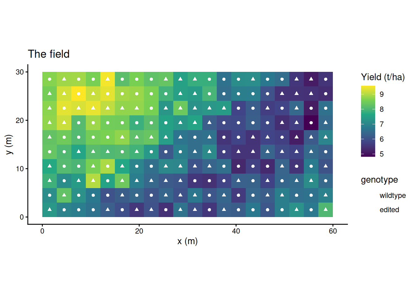

surf <- expand.grid(x_m = seq(1.5, 58.5, by = 1), y_m = seq(1.5, 28.5, by = 1), genotype = "wildtype")
surf$fit <- predict(m_sp, surf)
ggplot(surf, aes(x_m, y_m)) +
  geom_raster(aes(fill = fit)) +
  geom_contour(aes(z = fit), colour = "white", alpha = 0.6) +
  scale_fill_viridis_c() +
  coord_fixed() +
  labs(x = "x (m)", y = "y (m)", fill = "Fitted yield\n(t/ha)", title = "s(x_m, y_m): the fitted surface") +
  theme_classic()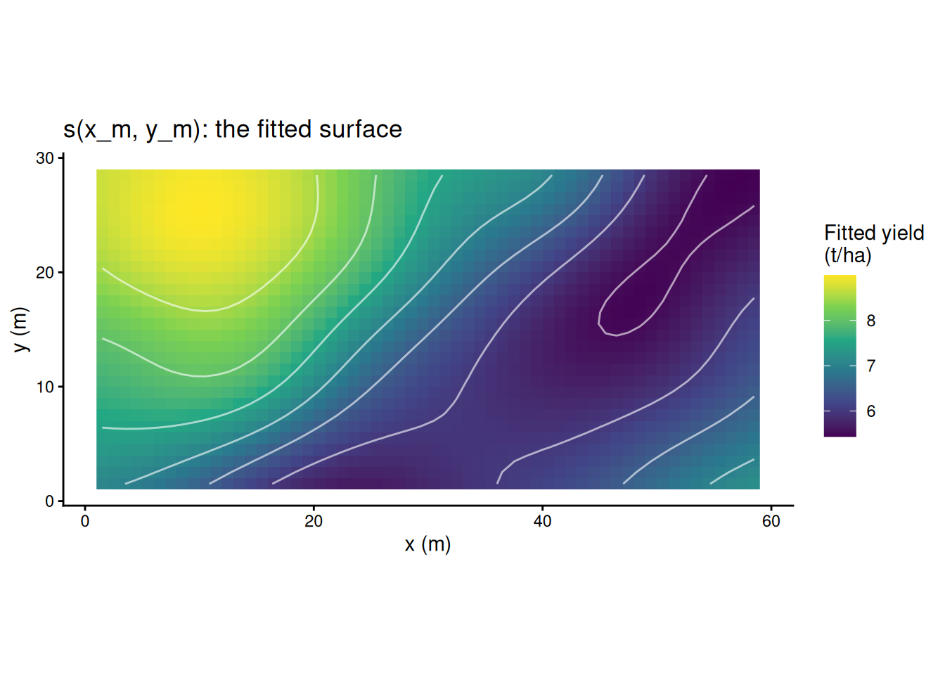

# the genotype effect with a 95% CI, both models
eff <- data.frame(model = c("lm(yield ~ genotype)", "gam(yield ~ genotype + s(x_m, y_m))"),
                  est = c(coef(m_naive)[2], coef(m_sp)[2]),
                  se = c(coef(summary(m_naive))[2, 2], summary(m_sp)$p.table[2, 2]))
ggplot(eff, aes(est, model)) +
  geom_vline(xintercept = 0, linetype = 2) +
  geom_pointrange(aes(xmin = est - 1.96 * se, xmax = est + 1.96 * se), colour = "#0070C0") +
  labs(x = "Edited minus wild type (t/ha), 95% CI", y = NULL) +
  theme_classic()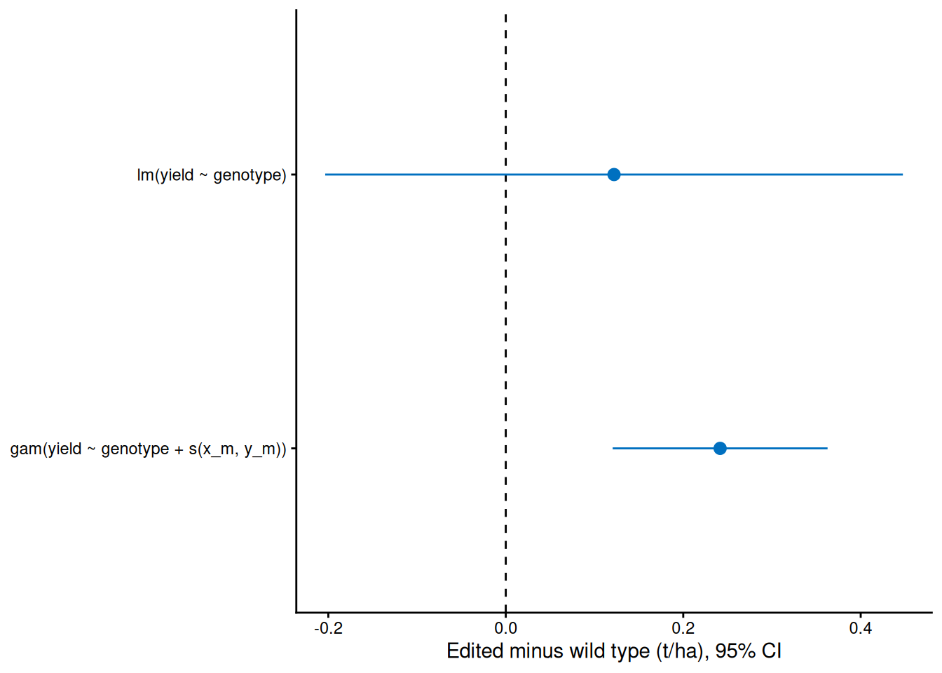

By chance more edited plots landed in poor patches, so the naive estimate is low and its SE is large. With the surface in the model, the estimate is close to the true 0.25 t/ha and the SE shrinks to about a third. Same data, same randomisation.

28) Different units: te()

s(x, y) treats both directions alike, which is right for two coordinates in metres. For predictors in different units (temperature and rainfall), use a tensor product smooth, te(), which gives each direction its own smoothness.

Demo: a simulated yield surface over temperature and rainfall

set.seed(35)
tr <- data.frame(temp = runif(250, 12, 34), rain_mm = runif(250, 200, 1200))
tr$yield <- 2 + 6 * exp(-((tr$temp - 24) / 6)^2) * (1 - exp(-tr$rain_mm / 400)) + rnorm(250, 0, 0.5)
m_te <- gam(yield ~ te(temp, rain_mm), data = tr, method = "REML")
summary(m_te)     # edf about 13.8


Family: gaussian 
Link function: identity 

Formula:
yield ~ te(temp, rain_mm)

Parametric coefficients:
            Estimate Std. Error t value Pr(>|t|)    
(Intercept)  4.39741    0.03289   133.7   <2e-16 ***
---
Signif. codes:  0 '***' 0.001 '**' 0.01 '*' 0.05 '.' 0.1 ' ' 1

Approximate significance of smooth terms:
                  edf Ref.df   F p-value    
te(temp,rain_mm) 13.8  16.06 157  <2e-16 ***
---
Signif. codes:  0 '***' 0.001 '**' 0.01 '*' 0.05 '.' 0.1 ' ' 1

R-sq.(adj) =   0.91   Deviance explained = 91.5%
-REML = 212.07  Scale est. = 0.27042   n = 250

Demo: a simulated yield surface over temperature and rainfall

gte <- expand.grid(temp = seq(12, 34, length.out = 60), rain_mm = seq(200, 1200, length.out = 60))
gte$fit <- predict(m_te, gte)
ggplot(gte, aes(temp, rain_mm)) +
  geom_raster(aes(fill = fit)) +
  geom_contour(aes(z = fit), colour = "white", alpha = 0.6) +
  scale_fill_viridis_c() +
  labs(x = "Temperature (°C)", y = "Rainfall (mm)", fill = "Fitted yield\n(t/ha)") +
  theme_classic()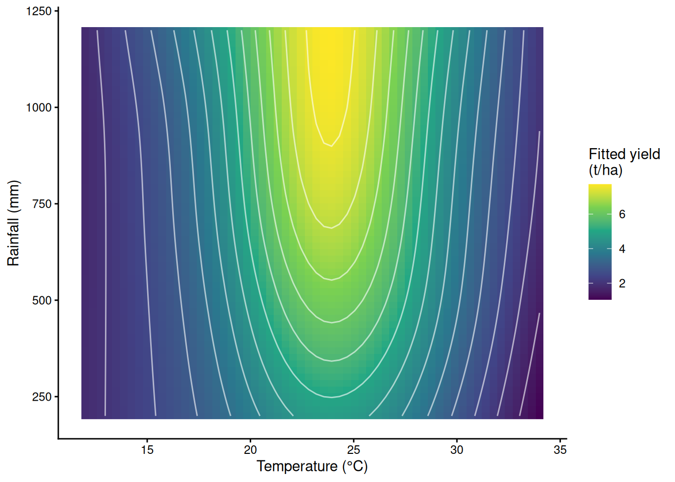

Part F. Mechanistic models with nls()

29) The maize N-rate trial and the quadratic optimum

8 nitrogen rates (0 to 280 kg N/ha) x 6 plots, grain yield in t/ha. Simulated. How much nitrogen is enough?

maize <- read.csv("https://greymonroe.github.io/PLS_206/data/maize_nitrogen.csv")
head(maize)

  plot N_rate yield
1    1    240 10.54
2    2    280 11.61
3    3    240 11.08
4    4    200 11.08
5    5    240 11.04
6    6      0  4.06

m_mq <- lm(yield ~ N_rate + I(N_rate^2), data = maize)
round(coef(summary(m_mq)), 6)

             Estimate Std. Error   t value Pr(>|t|)
(Intercept)  4.366597   0.208624  20.93046        0
N_rate       0.061527   0.003481  17.67639        0
I(N_rate^2) -0.000140   0.000012 -11.71053        0

bm <- coef(m_mq)
-bm[2] / (2 * bm[3])         # the quadratic's "optimum", about 220 kg N/ha

  N_rate 
219.7785

30) Linear-plateau with nls(): starting values from the plot

yield = a + b · min(N, N_c): a is the yield with no nitrogen, b the extra yield per kg N, and N_c the break point where the plateau starts (plateau = a + b · N_c). It is non-linear in N_c, so lm() cannot fit it: nls() (non-linear least squares) searches for the parameters step by step from a starting guess. Read the guesses off the plot: yield at 0 N is about 4.5 to 5, it rises about 6 t/ha over the first 150 kg (about 0.04 per kg), and the plateau starts somewhere near 150.

ggplot(maize, aes(N_rate, yield)) +
  geom_point(colour = "grey40") +
  labs(x = "Nitrogen rate (kg N/ha)", y = "Grain yield (t/ha)") +
  theme_classic()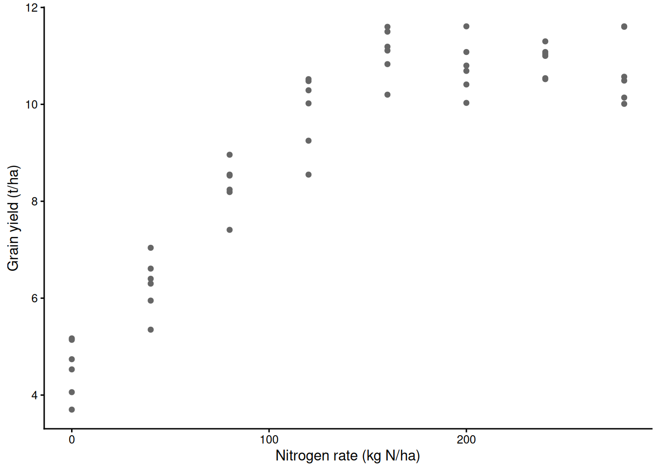

m_lp <- nls(yield ~ a + b * pmin(N_rate, Nc), data = maize,
            start = list(a = 5, b = 0.04, Nc = 150))
summary(m_lp)                # N_c about 141 kg N/ha


Formula: yield ~ a + b * pmin(N_rate, Nc)

Parameters:
    Estimate Std. Error t value Pr(>|t|)    
a  4.561e+00  1.926e-01   23.68   <2e-16 ***
b  4.481e-02  2.574e-03   17.41   <2e-16 ***
Nc 1.409e+02  5.898e+00   23.89   <2e-16 ***
---
Signif. codes:  0 '***' 0.001 '**' 0.01 '*' 0.05 '.' 0.1 ' ' 1

Residual standard error: 0.564 on 45 degrees of freedom

Number of iterations to convergence: 2 
Achieved convergence tolerance: 2.187e-09

Demo: a bad start, and the error it gives

bad <- try(nls(yield ~ a + b * pmin(N_rate, Nc), data = maize,
               start = list(a = 5, b = 0.04, Nc = 400)))   # break point beyond all the data

Error in nlsModel(formula, mf, start, wts, scaleOffset = scOff, nDcentral = nDcntr) : 
  singular gradient matrix at initial parameter estimates

With the break point guessed beyond the data, min(N, N_c) is just N for every plot, the model cannot tell N_c from anything else, and nls() stops. The fix is almost always better starting values, read off a plot. If a model refuses to converge from sensible starts, the data may not support that shape (a quadratic-plateau model on these data is one example).

31) Confidence intervals for parameters

confint() on an nls() fit profiles each parameter, which handles curved likelihoods better than ± 2 SE.

confint(m_lp)                # 95% CI for N_c: about 130 to 154 kg N/ha

           2.5%       97.5%
a    4.17268886   4.9486445
b    0.03962376   0.0499929
Nc 129.96182740 153.9820056

coef(m_lp)["a"] + coef(m_lp)["b"] * coef(m_lp)["Nc"]   # the plateau yield, t/ha

       a 
10.87292

32) Plotting an nls fit with a 95% CI

predict() on an nls() model gives no standard errors. nls_ci() builds them with the delta method: the gradient of the fitted curve with respect to each parameter (by a small numerical step), combined with the parameters’ covariance matrix.

nls_ci <- function(model, newdata, level = 0.95) {
  rhs <- formula(model)[[3]]
  f <- function(b) as.numeric(eval(rhs, c(as.list(newdata), as.list(b))))
  b <- coef(model); fit <- f(b)
  J <- sapply(seq_along(b), function(j) {        # numerical gradient, one column per parameter
    h <- 1e-6 * max(1, abs(b[j])); bj <- b; bj[j] <- bj[j] + h
    (f(bj) - fit) / h
  })
  se <- sqrt(rowSums((J %*% vcov(model)) * J))
  q <- qt(1 - (1 - level) / 2, df.residual(model))
  data.frame(newdata, fit = fit, lwr = fit - q * se, upr = fit + q * se)
}
g_N <- data.frame(N_rate = seq(0, 280, by = 1))
ci_lp <- nls_ci(m_lp, g_N)
ci_mq <- fit_ci(m_mq, g_N)
ggplot(maize, aes(N_rate, yield)) +
  geom_point(colour = "grey40") +
  geom_ribbon(data = ci_mq, aes(N_rate, ymin = lwr, ymax = upr), inherit.aes = FALSE, fill = "grey50", alpha = 0.15) +
  geom_line(data = ci_mq, aes(N_rate, fit), colour = "grey50", linetype = 2) +
  geom_ribbon(data = ci_lp, aes(N_rate, ymin = lwr, ymax = upr), inherit.aes = FALSE, fill = "red", alpha = 0.2) +
  geom_line(data = ci_lp, aes(N_rate, fit), colour = "red", linewidth = 1) +
  geom_vline(xintercept = coef(m_lp)["Nc"], colour = "red", linetype = 3) +
  geom_vline(xintercept = -bm[2] / (2 * bm[3]), colour = "grey50", linetype = 3) +
  labs(x = "Nitrogen rate (kg N/ha)", y = "Grain yield (t/ha)",
       subtitle = "red: linear-plateau (nls); dashed grey: quadratic") +
  theme_classic()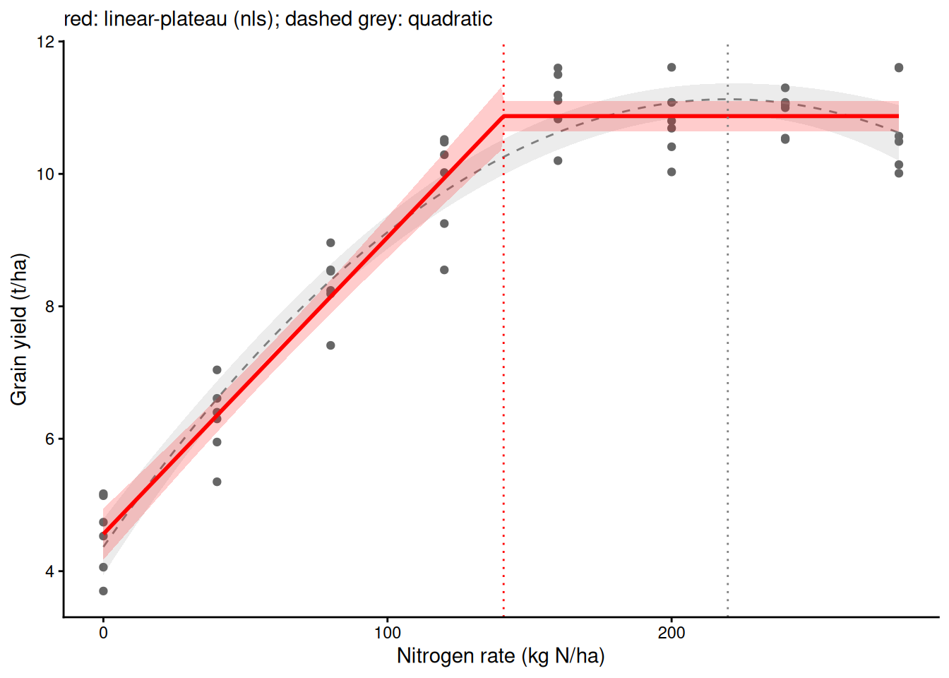

-bm[2] / (2 * bm[3]) - coef(m_lp)["Nc"]   # the quadratic overshoots by about 79 kg N/ha

  N_rate 
78.90628

33) Other mechanistic shapes

Each shape below has parameters with a biological meaning. Simulated curves for illustration.

Logistic growth: mass = Asym / (1 + exp((xmid − t) / scal)). Asym = final size, xmid = time of half size (fastest growth), scal = time scale of the rise. SSlogis() is a self-starting version that finds its own starting values.
Light response (exponential form): A = Amax · (1 − exp(−α · PAR / Amax)) − Rd. Amax = maximum gross photosynthesis (net photosynthesis levels off at Amax − Rd), α = initial slope (quantum efficiency), Rd = dark respiration.
Dose-response: a log-logistic curve with an EC50, the dose that halves the response. The drc package specialises in these.

set.seed(33)
grow <- data.frame(day = rep(seq(5, 80, by = 5), each = 3))
grow$mass <- 100 / (1 + exp((40 - grow$day) / 7)) * exp(rnorm(nrow(grow), 0, 0.1))
m_log <- nls(mass ~ SSlogis(day, Asym, xmid, scal), data = grow)   # no start needed
round(coef(summary(m_log)), 3)

     Estimate Std. Error t value Pr(>|t|)
Asym  101.860      1.764  57.755        0
xmid   39.894      0.590  67.652        0
scal    6.840      0.495  13.826        0

ci_log <- nls_ci(m_log, data.frame(day = seq(5, 80, by = 0.5)))
ggplot(grow, aes(day, mass)) +
  geom_point(colour = "grey40") +
  geom_ribbon(data = ci_log, aes(day, ymin = lwr, ymax = upr), inherit.aes = FALSE, fill = "darkgreen", alpha = 0.2) +
  geom_line(data = ci_log, aes(day, fit), colour = "darkgreen", linewidth = 1) +
  labs(x = "Day", y = "Mass (g)") +
  theme_classic()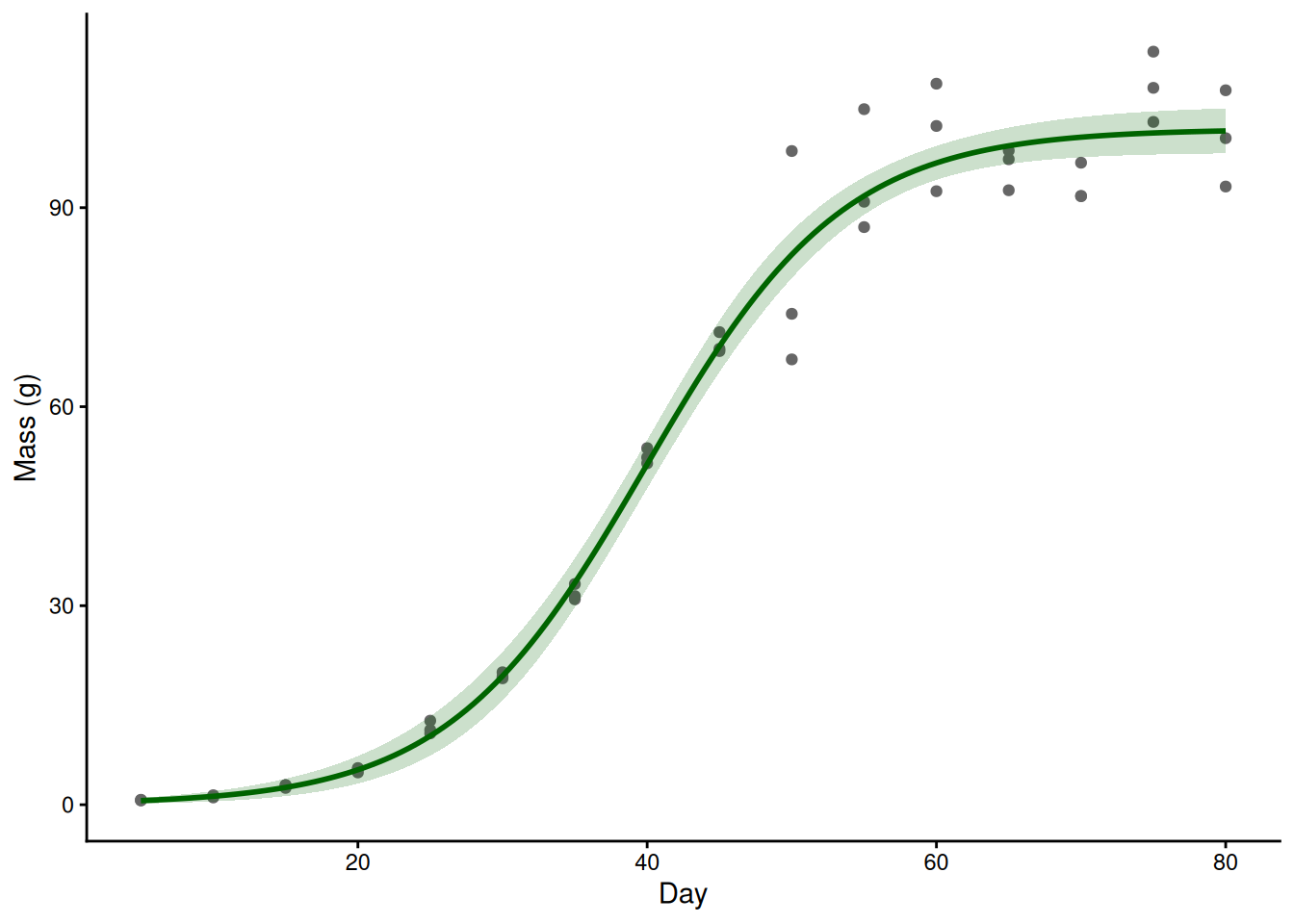

# a light-response curve: same pattern, with starting values read from a plot
set.seed(34)
leaf <- data.frame(PAR = rep(c(0, 50, 100, 200, 400, 700, 1000, 1500, 2000), each = 4))
leaf$A <- 20 * (1 - exp(-0.05 * leaf$PAR / 20)) - 1.5 + rnorm(nrow(leaf), 0, 1)
m_light <- nls(A ~ Amax * (1 - exp(-alpha * PAR / Amax)) - Rd, data = leaf,
               start = list(Amax = 18, alpha = 0.04, Rd = 1))
round(coef(summary(m_light)), 3)

      Estimate Std. Error t value Pr(>|t|)
Amax    19.835      0.452  43.912    0.000
alpha    0.049      0.003  14.521    0.000
Rd       1.382      0.362   3.817    0.001

ci_light <- nls_ci(m_light, data.frame(PAR = seq(0, 2000, by = 10)))
ggplot(leaf, aes(PAR, A)) +
  geom_point(colour = "grey40") +
  geom_ribbon(data = ci_light, aes(PAR, ymin = lwr, ymax = upr), inherit.aes = FALSE, fill = "orange", alpha = 0.3) +
  geom_line(data = ci_light, aes(PAR, fit), colour = "darkorange", linewidth = 1) +
  labs(x = expression(PAR~(mu*mol~photons~m^-2~s^-1)), y = expression(A~(mu*mol~CO[2]~m^-2~s^-1))) +
  theme_classic()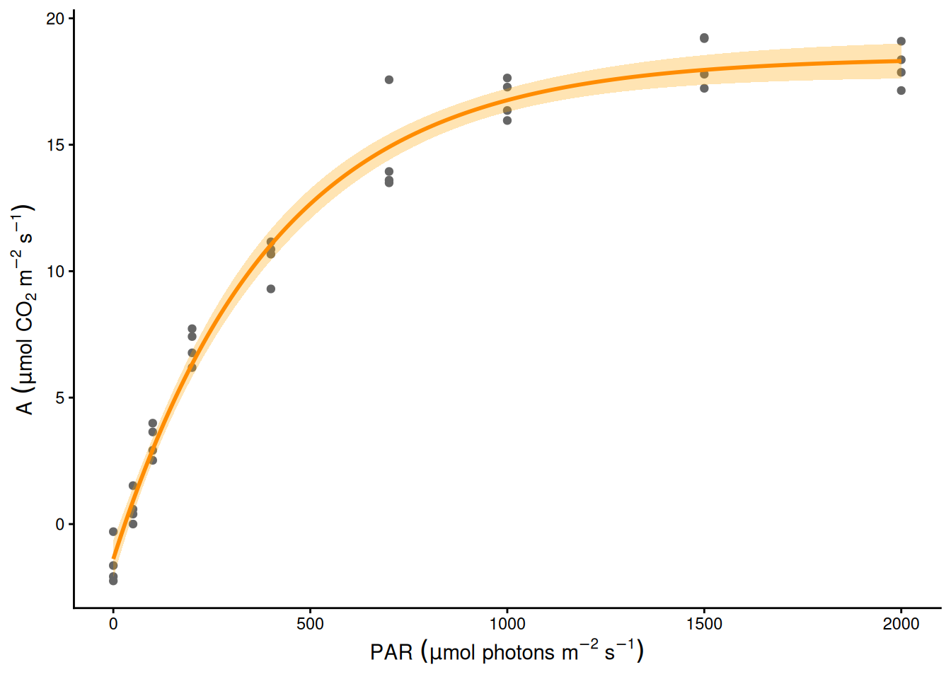

34) Describe or estimate: GAM vs nls on the same data

If you don’t know the shape and want the data to describe it, use a GAM. If theory gives a shape whose parameters answer your question, use nls() and report the parameters with CIs. Often both: the GAM to check the shape, nls() for the number. (Only 8 distinct N rates, so k = 8 is the most this smooth can have.)

m_mg <- gam(yield ~ s(N_rate, k = 8), data = maize, method = "REML")
summary(m_mg)        # describes the shape; no parameter called "where yield stops rising"


Family: gaussian 
Link function: identity 

Formula:
yield ~ s(N_rate, k = 8)

Parametric coefficients:
            Estimate Std. Error t value Pr(>|t|)    
(Intercept)  9.06104    0.08333   108.7   <2e-16 ***
---
Signif. codes:  0 '***' 0.001 '**' 0.01 '*' 0.05 '.' 0.1 ' ' 1

Approximate significance of smooth terms:
            edf Ref.df     F p-value    
s(N_rate) 4.382   5.29 143.4  <2e-16 ***
---
Signif. codes:  0 '***' 0.001 '**' 0.01 '*' 0.05 '.' 0.1 ' ' 1

R-sq.(adj) =  0.942   Deviance explained = 94.7%
-REML = 48.103  Scale est. = 0.33328   n = 48

ci_mg <- fit_ci(m_mg, g_N)
ci_both <- rbind(cbind(ci_mg[, c("N_rate", "fit", "lwr", "upr")], model = "GAM: describes the shape"),
                 cbind(ci_lp[, c("N_rate", "fit", "lwr", "upr")], model = "nls: estimates N_c"))
Nc_ci <- confint(m_lp)["Nc", ]
ggplot(maize, aes(N_rate, yield)) +
  geom_point(colour = "grey40") +
  geom_ribbon(data = ci_both, aes(N_rate, ymin = lwr, ymax = upr), inherit.aes = FALSE, fill = "blue", alpha = 0.2) +
  geom_line(data = ci_both, aes(N_rate, fit), colour = "blue", linewidth = 1) +
  geom_errorbar(data = data.frame(model = "nls: estimates N_c", xmin = Nc_ci[1], xmax = Nc_ci[2], y = 6),
                aes(xmin = xmin, xmax = xmax, y = y), inherit.aes = FALSE, colour = "red", width = 0.3,
                orientation = "y") +
  geom_text(data = data.frame(model = "nls: estimates N_c", x = mean(Nc_ci), y = 6.6, label = "95% CI for N_c"),
            aes(x, y, label = label), inherit.aes = FALSE, colour = "red", size = 3.5) +
  facet_wrap(~ model) +
  labs(x = "Nitrogen rate (kg N/ha)", y = "Grain yield (t/ha)") +
  theme_classic()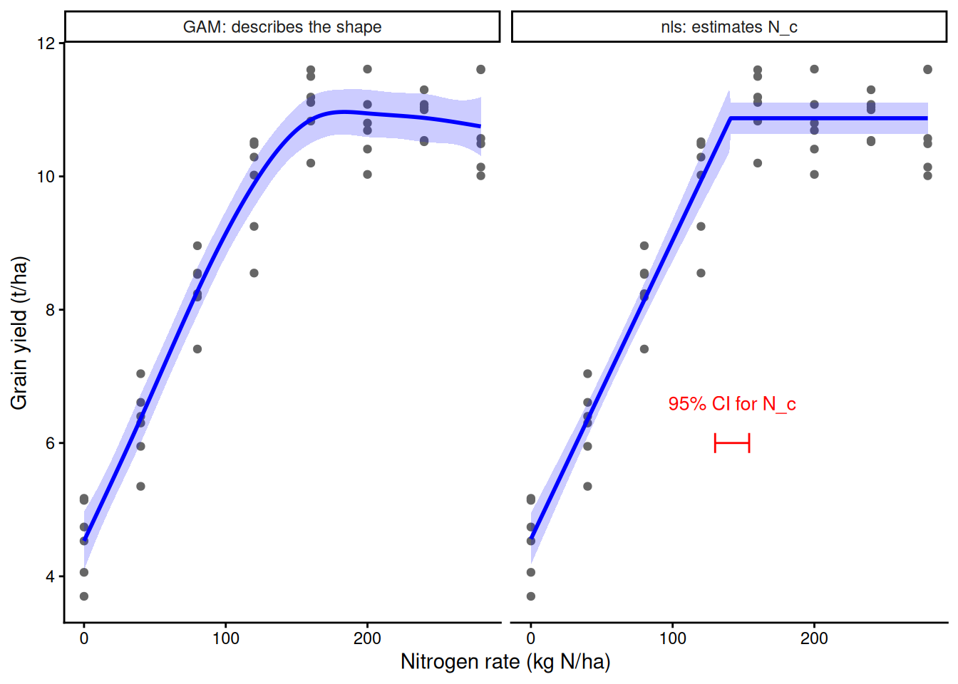

Example results sentence: Yield rose linearly by 0.045 t/ha per kg N (95% CI 0.040 to 0.050) up to a break point of 141 kg N/ha (95% CI 130 to 154), above which it was flat at 10.9 t/ha (linear-plateau model fitted with nls, n = 48).